Standard Deviation Differences Between Excel and R (and my code in Cube Voyager)
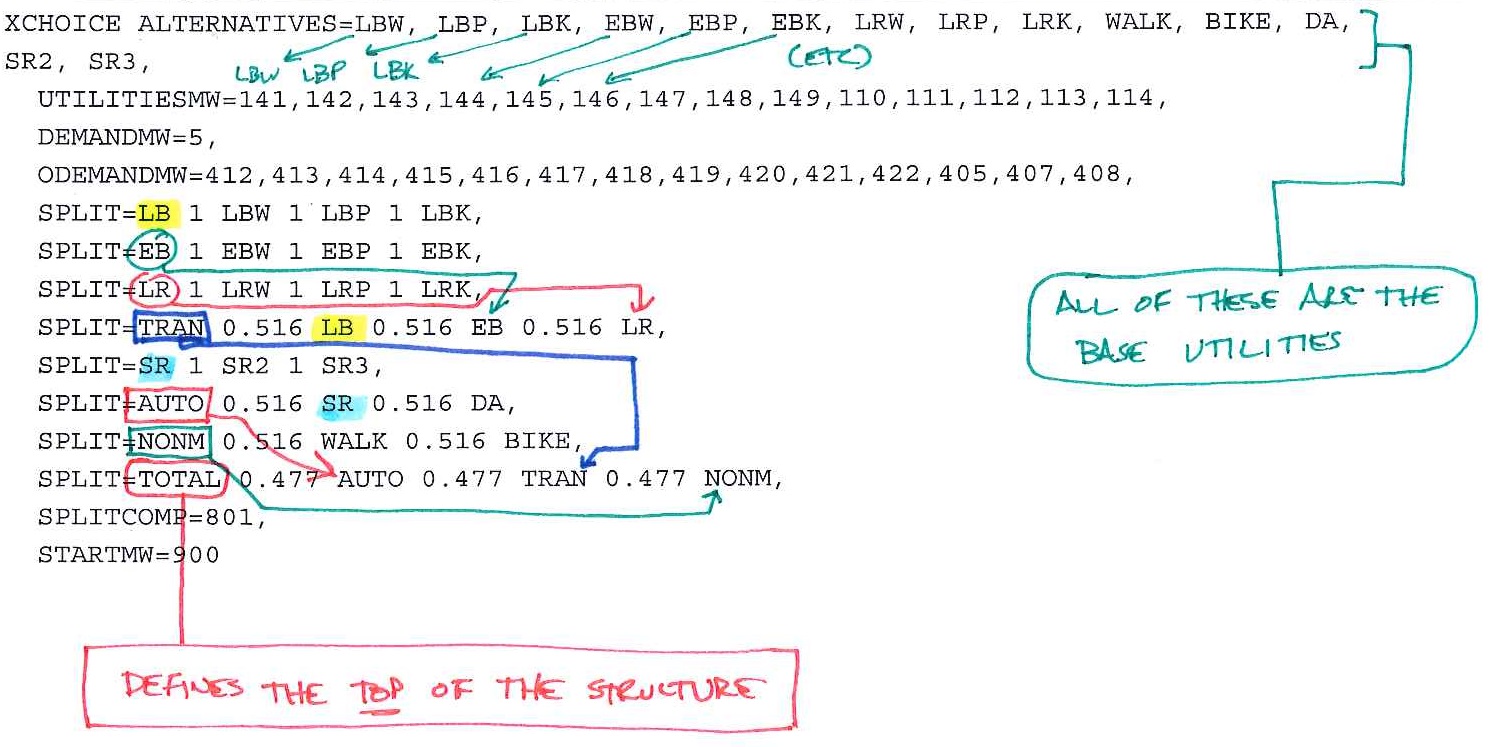
July 24th, 2015

I had a need to get the correlation of count to assignment in Cube Voyager. I don’t know how to do this off the top of my head, and I’m instantly mistrusting of doing things I’d normally trust to R or Excel. So I looked on Wikipedia for the Pearson product-moment correlation coefficient and ended up at Standard Deviation. I didn’t make it that far down on the page and used the first, which generally made Voyager Code like this:

I left the print statements in, because the output is important.

Avg AADT_TRK = 1121.77
Avg VOLUME = 822.03
n = 230.00


sdx1 = 1588160175
sdy1 = 1196330474
n = 230.00
sd AADT_TRK = 2627.75
sd Volume = 2280.67
r2 = 155.06

Note the standard deviations above. Ignore the R2 because it’s most certainly not correct!

Again, mistrusting my own calculations, I imported the DBF into R and looked at the standard deviations:

> sd(trkIn$AADT_TRK)
[1] 2633.476
> sd(trkIn$V_1)
[1] 2285.64

Now Standard Deviation is pretty easy to compute. So WHY ARE THESE DIFFERENT?

Just for fun, I did the same in Excel:

Screenshot 2015-07-24 11.09.18
WTF? Am I right or wrong???

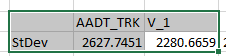
So I started looking into it and recalled something about n vs. n-1 in the RMSE equation and discussion in the latest Model Validation and Reasonableness Checking Manual. So I decided to manually code the standard deviation in Excel and use sqrt(sum(x-xavg)^2/n-1) instead of Excel’s function:

Looky there!  Matching Numbers!
Looky there! Matching Numbers!

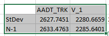
It’s not that Excel is incorrect, it’s not using Bessel’s Correction. R is.

/A

Lookups in R: The REAL Right Way!

September 9th, 2014

After waiting forever enough to get things to run, I stepped into a better way to do lookups.

mapply on matrix objects.

Basically, I do this:

TSkimLBWPk<-read.dbf("data/TSPKLBW.DBF") #Read the local bus walk skim

TSKimLBWPK_IWAIT=(acast(TSkimLBWPk,I~J,value.var="V1",drop=FALSE,fill=0)) #build a matrix from the data

TSKimLBWPK.IWAIT<-function(i,j) {
if(i<=nrow(TSKimLBWPK_IWAIT) && j<=ncol(TSKimLBWPK_IWAIT))
return(TSKimLBWPK_IWAIT[i,j])
else return(0)
} #build a function to lookup, returning 0 if it is looking for a zone not found

TripsAllPk$LBW.IWAIT=mapply(TSKimLBWPK.IWAIT,TripsAllPk$PTAZ,TripsAllPk$ATAZ) #do the lookup

That’s it. This takes the input DBF (which has I, J, V1, V2, etc. fields), converts to a matrix for a quick lookup, and then applies it.

It runs in about 3 minutes.

Lookups in R: The Wrong Way and the Right Way

August 28th, 2014

I recently wrote a script that takes DBF exports of Cube matrices and prepares them for Biogeme.  The main… well, only reason I did this in R was because I was considering using mlogit for model estimation.  I ultimately decided to ‘go with what I know’ and changed course to use Biogeme. Mind you, the part of Stairway to Heaven applies: “There are two paths you can go by, but in the long run / There’s still time to change the road you’re on.”

The Wrong Way

I’ve changed my code already, so pardon that this is from memory.  Also, these are snippets – I have a lot more code than this.

HSkimPk<-read.dbf("data/HSKIM_PK3.dbf")

for(rn in 1:nrow(TripsAll)){
HSkimPkRow<-subset(HSkimPk,I==TripsAll[rn,"PTAZ"] & J==TripsAll[rn,"ATAZ")
TripsAll$DA.IVT<-HSkimPkRow[,"V1"]
...
}

This took no less than 17 hours to complete for around 23,000 trip records and for values from 5 different tables * 2 time periods.

The Right Way

I (obviously) wanted something that wouldn't take forever, especially as I was working in Biogeme and seeing things that made me think that I wanted to change ONE LITTLE THING.  This seems to always happen.

I took a different approach that by my calculations should be much quicker.

HSkimPk<-read.dbf("data/HSKIM_PK3.dbf")
HSkimPkD<-acast(HSkimPk,I ~ J,value.var="V2",drop=FALSE,fill=0)
HSkimPkT<-acast(HSkimPk,I ~ J,value.var="V1",drop=FALSE,fill=0)

for(rn in 1:nrow(TripsAll)){
if(I<=nrow(HSkimPkT) & J<=nrow(HSkimPkT)){
TripsAll[rn,"DA.IVT"]<-HSkimPkT[I,J]
}
}

Since this is currently running, my only metrics are to look at the time per 50 rows (in my real code, I have a line that outputs a timestamp every 50 rows), and it is taking about 0.27 seconds per record, compared to somewhere around 4.5 seconds per record.  While not perfect, I'll take an estimated completion of 1.75 hours compared to 17 (update: 2 hours).  However, I will say that Cube is faster in this regard and that I may not have the fastest R solution.

Quick Cube Voyager Trick: Arrays

December 24th, 2013

While injecting bugs into a script, I found a quick trick in Cube related to arrays.  I didn’t test it to see if it works on a single-dimension array, but it DOES work on a multi-dimension array.

ARRAY Test=8,8

Test=1

This sets everything in Test to 1, so if you write:

LOOP _x=1,8

LOOP _y=1,8

PRINT LIST=Test[_x][_y]

ENDLOOP

ENDLOOP

The response will be ‘1’ 64 times.


Travel Model Reports with R and knitr

November 12th, 2013

I’ve had my share of complaining about the various “reporting” platforms available to those of us that do travel modeling.  I’ve looked at a few options, and nothing has stuck as “the one”. Until now.

In the meantime, I’ve noticed that a lot of groups have adopted Markdown.  It’s found it’s way onto Github via Jekyll.  Jeckyll’s found it’s way into my life as a quick blogging and site-building solution.  Then, I stumbled upon RStudio RMarkdown.  This is becoming a goldmine because RStudio is a great platform for developing things in R (including presentations and R Markdown).  Even better, the RMarkdown documents can be run via R (in a batch wrapper).  The only missing link is the ability to read matrix files directly.  I guess we can’t have everything, but I have a solution for that, too.

What Is This Markdown Thing And Why Should I Care?

Markdown is a pretty easy thing to grasp.  It’s open and fairly flexible.  It’s a text markup format that is easy to read when not rendered.  Easy to read means easy to write.  The open-ness means that you can do things with it.  In the case of RMarkdown, you can add R code blocks and LaTeX equations.  I will admit that LaTeX equations are not legible until rendered, but when you start adding R in the equation, the focus shifts less on reading the unrendered RMarkdown and more on reading the rendered output.

The link to Github (above) goes to their Markdown cheat sheet.  That alternates between Markdown and HTML output and it’s pretty easy to see how things work.

Getting Model Run Results into RMarkdown and into Rendered Output

There’s a number of things that need to happen to get model run results into R/RMarkdown and then to Output:

  1. Output data to a format R understands
  2. Write RMarkdown document
  3. Write RScript to render RMarkdown to HTML
  4. Write Windows Batch File to automate the RScript

Output data to a format R understands

In the case of zonal data, R can understand CSV out of the box, and with the appropriate library, can understand DBF.  With matrix files, Voyager will export them to DBF with a simple script file:

This script simply reads a bunch of matrix files and outputs them to two DBF files, one for the peak-period distribution and one for the off-peak-period distribution.

One important thing to note in this is that I didn’t put paths in this.  I run this from the command line in the model folder and it picks up the files in that folder and outputs the DBFs into that folder.  This is something that would have to be testing when placed into a model run file.

Resist the urge to do this in two separate steps.  The join process in R takes forever, and reading the data into memory may take a while, too.

Write RMarkdown document

The RMarkdown document is where the magic happens.  Fortunately, Knitr (the R Package that does all this magic) does a few things to split code blocks.  If you want to build my file, add all these together into one file and name it something.rmd

There are three code blocks that do this.  They are importing, summarizing, and graphing.

Importing Data

This block does three things:

  1. Loads libraries.  The foreign library is used to read DBF files.  The plyr library is used to join and summarize the data frames (from the DBF inputs).  The ggplot2 library is used for plots.
  2. Sets a few variables.  Since the OKI model is actually two MPO models, we do three reports of everything – one for the entire model, one for the OKI (Cincinnati) region, and one for the MVRPC (Dayton) region.  zones_oki and zones_mv are used to control which report is which.
  3. Imports the DBF files.  Those read.dbf lines are where that magic happens.  Again, since this is run in the model folder, no paths are used.

Summarizing Data

This block does three things:

  1. It rounds the logsum values to provide some grouping to the values
  2. It gets a subset of the model (for OKI)
  3. It summarizes the rounded values to prepare for charting them

Charting Data

This block does one thing: it draws the chart using the ggplot tool.  This is pretty advanced (although not bad, and the online help is good).  However, for this I’m going to hold to my recommendation to get a copy of The R Graphics Cookbook (where I learned how to use ggplot).  The concepts and examples in the book are far greater than what I will post here.

One point that should not be lost is that text elements (either Markdown headings, etc., or just text, or formatted text) can be added into this outside of the “`…“` blocks. This way, reports can actually look good!

Once this part is complete, the hardest stuff is over.

Write RScript to render RMarkdown to HTML

The RScript to render the RMarkdown file to HTML is pretty simple:

This writes the .Rmd file out to the same filename as .html. You can have as many knit2html lines as needed

There are ways to write the files out to PDF (I haven’t looked into them… perhaps that would be a future blog topic?).

Write Windows Batch File to automate the RScript

The last step is to write a batch file “wrapper” that can be run as part of the travel demand model run.  This is really quite easy:

The first line sets the path to include R (on my system it isn’t in the path, and my path statement is already 9 miles long). The second line runs the R script file (ReportR.R) in R.


That’s It! It seems like a lot of work goes into this, but it isn’t as difficult as some of the other reporting platforms out there.

PS: Stay tuned for some example reports

Update:

Example Report (generated from RMarkdown file)

Example RMarkdown File

AutoHotKey + Cube Voyager: Curly Braces

October 29th, 2013

I am rebuilding the mode choice and distribution parts of the OKI model (that may be obvious from the last two or three posts on this blog), and decided to use AutoHotKey to speed things up.  I wanted to add the MO=… NAME=… and AUTOMDARRAY lines to the MATO and two DBI lines:

^!o::Send MO=101-117 NAME=LBW,LBP,LBK,EBW,EBP,EBK,LRW,LRP,LRK,Walk,Bike,DA,SR2,SR3,CRW,CRP,CRK
^!1::Send AUTOMDARRAY=PCWALK INDEXES=TAZ-{ZONES_MV} ARRAYFIELDS=PRODSWOP, ATTRSWOP, PRODLWOP, ATTRLWOP
^!2::Send AUTOMDARRAY=MSEG INDEXES=NDSTX-{ZONES_MV} ARRAYFIELDS=HBW1,HBW2,HBW3,HBW4,COCODE

In the OKI model, {ZONES_MV} is all internal zones. I used this, did some other copy and paste magic, and was greeted with the errors:


F(795): DBI[2] ARRAYFIELDS=NDSTX must have a valid numeric size specified (-#)

F(795): DBI[1] ARRAYFIELDS=TAZ must have a valid numeric size specified (-#)

It seems the curly braces aren’t immediately cool with AHK.

The solution (per this post, and it works) is to enclose the curly braces in curly braces:

^!1::Send AUTOMDARRAY=PCWALK INDEXES=TAZ-{{}ZONES_MV{}} ARRAYFIELDS=PRODSWOP, ATTRSWOP, PRODLWOP, ATTRLWOP
^!2::Send AUTOMDARRAY=MSEG INDEXES=NDSTX-{{}ZONES_MV{}} ARRAYFIELDS=HBW1,HBW2,HBW3,HBW4,COCODE

Cube Voyager XCHOICE: The Missing Help Doc

October 22nd, 2013

First note: I sent this to the support people at Citilabs recently, so maybe on the next update they’ll include this in the help document, as I think it is sorely missing.  Or maybe I’m just crazy (you kinda have to be crazy to do transportation modeling*) and have my own way of thinking.

In the OKI model, we have a nested logit mode choice structure that’s pretty common for MPOs our size – it’s had a history in several other MPOs.  The nesting structure looks like this:


OKI Mode Choice


The part that I think is missing in the Voyager Help File for XCHOICE is this:

XCHOICE ALTERNATIVES=LBW, LBP, LBK, EBW, EBP, EBK, LRW, LRP, LRK, WALK, BIKE, DA, SR2, SR3,
UTILITIESMW=141,142,143,144,145,146,147,148,149,110,111,112,113,114,
DEMANDMW=5,
ODEMANDMW=412,413,414,415,416,417,418,419,420,421,422,405,407,408,
SPLIT=LB 1 LBW 1 LBP 1 LBK,
SPLIT=EB 1 EBW 1 EBP 1 EBK,
SPLIT=LR 1 LRW 1 LRP 1 LRK,
SPLIT=TRAN 0.516 LB 0.516 EB 0.516 LR,
SPLIT=SR 1 SR2 1 SR3,
SPLIT=AUTO 0.516 SR 0.516 DA,
SPLIT=NONM 0.516 WALK 0.516 BIKE,
SPLIT=TOTAL 0.477 AUTO 0.477 TRAN 0.477 NONM,
SPLITCOMP=801,
STARTMW=900

More importantly, WHY this is important:

XCHOICE

All those green, blue, red, and yellow marks are pointing things out – like what connects to what and so on.  Once these connections are made, you can get answers without a lot of effort.  It’s quite nice, really.  However, I haven’t figured out where to put upper-level coefficients, but in my latest estimation runs, those are out.

More Stuff

One of the more important things to get out of the mode choice model is the logsum values that would be used as the impedance for a gravity model distribution.  Once you have the above, it’s pretty easy.

First off, make your demand matrix have 100 trips per IJ pair:

MW[2]=100

Then, get the exponential of the SPLITCOMP matrix to get a usable logsum value.

MW[700]=EXP(MW[801])

Note that in the OKI model (and in other models that use walk access markets), this needs to be done multiple times and accumulated to another matrix:

MW[701]=MW[701]+(MW[5]*MW[700])

And then there is some post-processing that needs to be done at the end of the ILOOP:

JLOOP
IF(MW[2]>0)
MW[702]=MW[701]/MW[2] ;Denom
ELSE
MW[702]=0.00000000001
ENDIF

MW[704]=(LN(MW[702])/(COEFF[1]*CLSPRM*CLSSUB))+LOGADD
ENDJLOOP

704 is the output matrix.

* I have other forms of craziness, too.  I’ve recently announced – and made it “Facebook official” to my close friends and family – that I’m going to run a half marathon next spring.

Reading and Analyzing Cube Voyager PT Route Trace Files

October 8th, 2013

After an unsuccessful attempt in trading mode choice calibration with bugfixing in Cube, I ended up figuring out several things about Voyager PT and route trace files.

Trace Reports

The trace reports are files that describe the transit routes from one zone to another.  This is a little more detailed than the skim matrices, as the skims don’t tell you which routes are used or the operator of the routes (since there are five transit providers in the OKI model, this is a major concern).  The trace reports look like this (this is from a subset of the OKI model):


REval Route(s) from Origin 10 to Destination 18

10 -> 4835
4835 -> 4839 -> 4865 lines Rt1IB Rt10IB Rt10OB Rt28MOB Rt32IB Rt27IB
4865 -> 4859 -> 18 lines Rt5TankOB Rt5TankIB Rt7TankOB Rt7TankIB Rt9TankIB Rt9TankOB Rt11TankIB Rt16TankIB Rt23TankIB Rt25TankIB
Cost= 65.11 Probability=1.0000

REval Route(s) from Origin 10 to Destination 19

10 -> 4835
4835 -> 4839 -> 19 lines Rt1IB Rt10IB Rt10OB Rt28MOB Rt32IB Rt27IB
Cost= 33.42 Probability=1.0000

REval Route(s) from Origin 10 to Destination 20

10 -> 4835
4835 -> 4839 -> 20 lines Rt1IB Rt10IB Rt10OB Rt28MOB Rt32IB Rt27IB
Cost= 33.42 Probability=1.0000

Voyager PT Setup

There is one thing that’s not really well documented in Cube Help, and that is how to generate the trace reports.  The one thing that has to be done is on the FILEI ROUTEI or FILEO ROUTEO lines, the line must include both REPORTI=z-Z and REPORTO=z-Z.  The report will not generate if only one side is there – both keys have to be there.  There must also be a FILEO REPORTO file, but that’s required for any Voyager PT run.

So What?

Having this was only half the battle.  I needed a matrix of the operator, and for the entire 3,200 (ish) zone model run, the resulting report file is over 1.2 GB (and that doesn’t include Dayton’s transit!).  So I had to go through this file quickly.  Enter Java.

I wrote a quick (both in code and in running) Java program to read the report file and a DBF of the lines (which I got from the geodatabase route layer). The program sorts through the report file looking for the excerpts above, stores them in memory, and then scans through them to output a dbf with the from-zone (I), to-zone (J), and the operator. This is multi-threaded, so on my 8-core beast, it runs very fast.

The Github repository is here.

Now, on to mode choice…

Taking CSV Exported Cube Voyager Path Files to A New Level Using GAWK (part 1)

January 30th, 2013

In a prior post, I link to some code that outputs a path file.  I’ve done something a tad different because I needed some select link analysis and reading the path file in Cube was taking far too long to do it the normal way.

So, I took that program on Github and extended it to perform a selected link:

And this outputs a few GB of paths in CSV format.  I went from 42 GB of paths in the AM to 3.4 GB of CSV paths.  Still not good enough. The next thing I did was use GAWK to get just the Origin and Destination

This returns a CSV file of just the origin and destination (which can be linked to the vehicle trip matrix).

Part 2 will discuss how to link to a vehicle trip matrix and if this approach actually works!

Reading a Cube Voyager Path File from Java

October 8th, 2012

As a follow-up to my prior post, this is how to use the Cube Voyager API to read a path file.  I highly recommend you read the other article first, as it talks more about what is going on here.

The Interface

The interface for the path reader is larger because of the return structure.  The code below includes the interfaces to the DLL calls and the structure for the path data returned by some of them.  Note that I didn’t do PathReaderReadDirect.  It doesn’t seem to work (or I’m not trying hard enough).

The Code

Once the interface is in place, the code is reasonably simple.  However, I’m seeing a few interesting things in the costs and volumes in both C++ and in Java, so I wouldn’t use those values.  I guess if you need to determine the costs, you should save the costs with the loaded highway network to a DBF file and read that into an array that can be used to store and get the values.

The Final Word… For Now

Java is a great programming language.  Using these DLLs can help you do some interesting stuff.  However, it seems that there are very few people using the API, which is concerning.  I personally would like to see an interface for reading .NET files and writing matrices.  But I can’t expect Citilabs to put time in on that when it seems there are so few people using it.


Reading a Cube Voyager Matrix from Java using JNA

October 5th, 2012

I’ve begun to really enjoy Java.  It’s hot, black exterior exposes a sweet bitterness that matches few other things in this world.  Oh, wait, this is supposed to be about the other Java – the programming language!

The “Holy Grail” of API programming with Cube Voyager to me has been using the API in Java.  I can program in C++ quite well, but I have a staff that can’t.  We’re likely going to be going to a Java based modeling structure in the next few years, so  it makes sense to write everything in Java and keep the model down to two languages – Cube Voyager and Java.

Setting up the Java Environment

There are three things to do to setup the Java environment to make this work.  The first is to place the Cube DLL in the right location.  The second is to get JNA and locate the libraries to where you need them.  The final is to setup the Java execution environment.

First, copy the VoyagerFileAccess.dll file (and probably it’s associated lib file) to C:\Windows.  It should work.  I’m using a Windows 7-64 bit machine, so if it doesn’t work, try C:\Windows\System32 and C:\Windows\System.

Second, get JNA.  This allows the Java compiler to connect to the DLL.  The latest version can be downloaded from Github (go down to “Downloads” under the Readme.md… just scroll down ’till you see it, and get both platform.jar and jna.jar).

If you’re on a 64-bit computer, the second thing to do is to set your jdk environment to use a 32-bit compiler.  I use Eclipse as my IDE, so this is done through the project properties.  One location is the Java Build Path – on the Libraries tab, make sure the JRE System Library is set to a 32-bit compiler.  In the Java Build Path screenshot below, you can see that all the locations are in C:\Program Files (x86) – this is an easy (although not foolproof) way to show that this is a 32-bit compiler.

Java Build Path Window

While you’re setting up stuff in this window, make sure the jna.jar and platform.jar are linked here as well (click “Add External JARs…” and locate those two files).

Another place to check in Eclipse is the Java Compiler settings, which should have “Use Compliance from execution environment…” checked.

The Programming

The thing that makes this work is this part of the programming.  You can see in this that I create an interface t0 the Voyager DLL file by loading the DLL, and then setup some pointer objects to hold the memory pointer variable (the “state” variable in all of these) and set up the functions to read from the matrix.

public interface voyagerDLL extends Library{
voyagerDLL INSTANCE=(voyagerDLL) Native.loadLibrary("VoyagerFileAccess",voyagerDLL.class);
Pointer MatReaderOpen(String filename, Pointer errMsg, int errBuffLen);
int MatReaderGetNumMats(Pointer state);
int MatReaderGetNumZones(Pointer state);
int MatReaderGetMatrixNames(Pointer state, String[] names);
int MatReaderGetRow(Pointer state, int MatNumber, int RowNumber, double[] buffer);
void MatReaderClose(Pointer state);
}

The next part that makes this work is the actual programming. In the code below, the first thing I do is define vdll as an instance of the voyagerDLL interface.  Then, I open a matrix file (yes, it is hard-coded, but this is an example!), get the number of matrices, zones, the names, and I start reading the matrix (in the for loops).  I only print every 100th value, as printing each one makes this slow a bit. The actual reading is quite fast.  Finally, I close the matrix and the program terminates.

Issues

The big issue I noticed is that if the matrix is not found, the Pointer variable returned by MatReaderOpen will be null, but nothing will be in the error value.  I’ve tried redefining the error value to be a string in the interface, but it does the same thing.  However, I don’t recall if it did anything in C++.  At any rate, there needs to be some error checking after the matrix is opened to ensure that it actually has opened, else the program will crash (and it doesn’t do a normal crash).

Next Up

The next thing I’m going to do is the path files.

Using the Voyager API for Path Analysis

August 3rd, 2012

Just posted on Github: Path2CSV

This is a tool that will read a Cube Voyager Path file and output the contents by node to a CSV file.  The code is written in C++ and available under the GPL3 license.


Interesting INT() Issue Between Cube and Excel

July 24th, 2012


I don’t know about anyone else, but I do a lot of calculation prototyping in Excel before applying that in scripts.  One of the most recent was to do a script to add expansion zones (also known as “dummy zones”, although they aren’t really dumb, just undeveloped!).

The problem I had was related to the following equation:

R=INT((819-N)/22)+1   Where N={820..906}

In Excel, the results are as below (click on it if it is too small to see):

In Cube, I got the result of (click on it to expand, and I only took it into Excel to move stuff around and make it easier to see):

Note the sheer number of zeroes in the Cube version and all the numbers are ‘off’.

The reason, as I looked into things was because of how INT() works differently in the two platforms.  In Cube, INT simply removes everything to the right of the decimal, so INT(-0.05) = 0, and INT(-1.05)=-1.  In Excel, INT rounds down to the nearest integer.  This means that negative values will be different between the two platforms.  Note the table below.

Excel Cube
3.4 3 3
2.3 2 2
1.1 3 1
0.5 0 0
0 0 0
-0.5 -1 0
-1.1 -2 -1
-2.3 -3 -2
-3.4 -4 -3

While neither software is truly wrong in it’s approach (there is no standard spec for INT()) it is important to know why things may not work as expected.

More Voyager PT + AWK Goodness

September 20th, 2011

One thing I’ve missed from the old TranPlan days was the reporting group.  We’ve used that for many years to compare our transit loadings by major corridor.  Unfortunately, that functionality was lost going to PT.  I still need it, though, and enter awk.

The script below looks at the transit line file and outputs ONLY the line code, comma-separated.  It uses a loop to check each field for ‘ NAME=’ and ‘USERN2’, which is where we now store our reporting group codes.

BEGIN{
FS=","
RS="LINE"
}
{
	for (i=1;i<20;i++)
	{
		if($i~/ NAME=/)
		{
			printf "%s,",substr($i,8,length($i)-8)
		}
		if($i~/USERN2/)
		{
			printf "%s\n",substr($i,9)
		}
	}
}

The contents of the above need to be saved to a .awk file - I used trn.awk.

To call this, I use a Pilot script to call awk and pass the input and get the output.

*awk -f {CATALOG_DIR}/INPUTS/trn.awk {CATALOG_DIR}/INPUTS/OKIROUTES.LIN >{CATALOG_DIR}/OKIROUTES.CSV

The output of this is a simple two-column comma-separated-value file of the route ID and the reporting group.

Using Gawk to get a SimpleTransit Loadings Table from Cube PT

September 19th, 2011

One thing that I don’t like about Cube is the transit loadings report is stuck in the big program print report.  To pull this out, the following code works pretty well:

gawk /'^REPORT LINES  UserClass=Total'/,/'^Total     '/ 63PTR00A.PRN >outputfile.txt

Where 63PTR00A.PRN is the print file. Note the spaces after ^Total. For whatever reason, using the karat (the ‘^’) isn’t working to find ‘Total’ as the first thing on the line. So, I added the spaces so it gets everything. Outputfile.txt is where this will go. It will just be the table.

NOTE: You need GNUWin32 installed to do this.

Using gawk to Get PT Unassigned Trips Output into a Matrix

July 15th, 2011

In the process of quality-control checking a transit on-board survey, one task that has been routinely mentioned on things like TMIP webinars is to assign your transit trip-table from your transit on-board survey.  This serves two purposes – to check the survey and to check the transit network.

PT (and TranPlan’s LOAD TRANSIT NETWORK, and probably TRNBUILD, too) will attempt to assign all trips.  Trips that are not assigned are output into the print file.  In PT (what this post will focus on), will output a line similar to this:


W(742): 1 Trips for I=211 to J=277, but no path for UserClass 1.

When a transit path is not found.  With a transit on-board survey, there may be a lot of these.  Therefore, less time spent writing code to parse them, the better.

To get this to a file that is easier to parse, start with your transit script, and add the following line near the top:


GLOBAL PAGEHEIGHT=32767

This removes the page headers. I had originally tried this with page headers in the print file, but it created problems. Really, you probably won’t print this anyway, so removing the page headers is probably a Godsend to you!

Then, open a command line, and type the following:

gawk '/(W\(742\).*)\./ {print $2,$5,$7}' TCPTR00A.PRN >UnassignedTransitTrips.PRN

Note that TCPTR00A.PRN is the transit assignment step print file, and UnassignedTransitTrips.PRN is the destination file. The {print $2,$5,$7} tells gawk to print the second, fifth, and seventh columns. Gawk figures out the columns itself based on spaces in the lines. The >UnassignedTransitTrips.PRN directs the output to that file, instead of listing it on the screen.

The UnassignedTransitTrips.PRN file should include something like:


1 I=3 J=285,
1 I=3 J=289,
1 I=3 J=292,
1 I=6 J=227,
1 I=7 J=1275,

The first column is the number of unassigned trips, the second column is the I zone, and the last column is the J zone.

This file can then be brought into two Matrix steps to move it to a matrix. The first step should include the following code:

RUN PGM=MATRIX PRNFILE="S:\USER\ROHNE\PROJECTS\TRANSIT OB SURVEY\TRAVELMODEL\MODEL\TCMAT00A.PRN"
FILEO RECO[1] = "S:\User\Rohne\Projects\Transit OB Survey\TravelModel\Model\Outputs\UnassignedAM.DBF",
 FIELDS=IZ,JZ,V
FILEI RECI = "S:\User\Rohne\Projects\Transit OB Survey\TravelModel\Model\UnassignedTransitTrips.PRN"

RO.V=RECI.NFIELD[1]
RO.IZ=SUBSTR(RECI.CFIELD[2],3,STRLEN(RECI.CFIELD[2])-2)
RO.JZ=SUBSTR(RECI.CFIELD[3],3,STRLEN(RECI.CFIELD[3])-2)
WRITE RECO=1

ENDRUN

This first step parses the I=, J=, and comma out of the file and inserts the I, J, and number of trips into a DBF file. This is naturally sorted by I then J because of the way PT works and because I am only using one user class in this case.

The second Matrix step is below:

RUN PGM=MATRIX
FILEO MATO[1] = "S:\User\Rohne\Projects\Transit OB Survey\TravelModel\Model\Outputs\UnassignedAM.MAT" MO=1
FILEI MATI[1] = "S:\User\Rohne\Projects\Transit OB Survey\TravelModel\Model\Outputs\UnassignedAM.DBF" PATTERN=IJM:V FIELDS=IZ,JZ,0,V

PAR ZONES=2425

MW[1]=MI.1.1
ENDRUN

This step simply reads the DBF file and puts it into a matrix.

At this point, you can easily draw desire lines to show the unassigned survey trips. Hopefully it looks better than mine!

Emailing an alert that a model run is complete in Cube Voyager

March 6th, 2011

When you are doing many model runs, it makes life easier to know if the modelrun is complete.  The code is below.

SENDMAIL,
SMTPSERVER='MAILSERVER HERE',
FROM='from@somwehere.com',
TO='to@somewhere.com',
SUBJECT='Subject Line Here',
MESSAGE='Message Goes Here',
USERNAME='username',
PASSWORD='password'

The things you replace here are pretty obvious.  If you have questions about the SMTPSERVER parameter, ask your IT person.  Also, for Windows domains, the USERNAME parameter should be ‘DOMAIN\USERNAME’ (you may be able to use your email address, depending on your email setup).

Python and Cube

December 19th, 2010

One of the advantages of the ESRI ArcGIS Framework is that you can write Python scripts that do GIS things and run them from Cube.  Even better, Cube uses the Geodatabase format, so you can store and retrieve things from there.

The first thing that is needed is a python script.  The below is an example that we’re not using at the moment, but it merges multiple transit line files together.

import arcgisscripting, sys, os
gp=arcgisscripting.create()

gp.AddToolbox("C:/Program Files/ArcGIS/ArcToolBox/Toolboxes/Data Management Tools.tbx")

print sys.argv

input1=sys.argv[1]
input2=sys.argv[2]
output=sys.argv[3]

in1=input1+input1[input1.rfind("\\"):]+"_PTLine"
in2=input2+input2[input2.rfind("\\"):]+"_PTLine"

input=in1+';'+in2
input=input.replace("\\","/")
output=output.replace("\\","/")

print input
print output

if gp.Exists(output):
    gp.delete_management(output)

#input=input1+"_PTLine" +';'+input2 +"_PTLine"

gp.Merge_management(input,output)

print gp.GetMessage

del gp

To call this, we add the following in a Pilot script:

*merge.py {CATALOG_DIR}\Inputs\Transit.mdb\Routes1 {CATALOG_DIR}\Inputs\Transit.mdb\Routes2 {CATALOG_DIR}\Inputs\Transit.mdb\RoutesCombined

This makes it easy to create geoprocessing steps in ArcMap, export them to Python, and call them from the model.

Using a Class Object to Help Read a Control File

December 5th, 2010

One thing we’re used to in travel modeling is control files.  It seems to harken back to the days of TranPlan where everything had a control file to control the steps.

In my case, I have a control file for my nested logit mode choice program, and because of the age of the mode choice program, I want to redesign it.  The first part of this is reading the control file, and I did a little trick to help with reading each control file line.  With C++, there is no way to read variables in from a file (like there is with FORTRAN).

The first part of the code reads the control file, and you will see that once I open and read the control file, I section it out (the control file has sections for files ($FILES), operation parameters ($PARAMS), operation options ($OPTIONS), and mode choice parameters ($PARMS). Each section ends with an end tag ($END). This adds the flexibility of being able to re-use variables in different locations.

After the section, the next portion of the code reads the line and checks to see if FPERIN is found. If it is, a ControlFileEntry object is created. This object is a class that is used to return the filename held in the object. This makes it easy to reduce code.

int readControlFile(char *controlFileName){
	cout << "Reading " << controlFileName << endl;
	//Read the control file
	string line;
	bool inFiles=false, inParams=false, inOptions=false, inParms=false;
	ifstream controlFile(controlFileName);
	if(!controlFile.good()){
		cout << "PROBLEMS READING CONTROL FILE" << endl;
		return 1;
	}
	while(controlFile.good()){
		getline(controlFile,line);
		//check the vars sections
		if(line.find("$FILES")!=string::npos)
			inFiles=true;
		if(line.find("$PARAMS")!=string::npos)
			inParams=true;
		if(line.find("$OPTIONS")!=string::npos)
			inOptions=true;
		if(line.find("$PARMS")!=string::npos)
			inParms=true;
		if(line.find("$END")!=string::npos){
			inFiles=false;
			inParams=false;
			inOptions=false;
			inParms=false;
		}
		if(inFiles){
			cout << "Checking files" << endl;
			if(line.find("FPERIN")!=string::npos){
				controlFileEntry cfe(line);
				PerTrpIn=cfe.filename;
			}
//SNIP!!!
	return 0;
}

The controlFileEntry is code is below.  This is used at the top of the code, just below the preprocessor directives (the #include stuff).

class controlFileEntry{
public:
	string filename;
	controlFileEntry(string Entry){
		beg=(int)Entry.find("=")+2;
		end=(int)Entry.rfind("\'")-beg;
		filename=Entry.substr(beg,end);
	}
	~controlFileEntry(){
		beg=0;
		end=0;
		filename="";
	}
private:
	string Entry;
	int beg;
	int end;
};

The class has one public member, filename, which is what is read in the code where it is used. There are two public functions. The first is the constructor (controlFileEntry) which is used when creating the object. The second is the de-constructor (~controlFileEntry), which sets the beg, end, and filename variables to zero and blank.  The beg, end (misnomer), and the line sent to it are private and cannot be used in code.

This can be extended, as the file entry type is fine when there are quotes around the item (it is setup for that, note the -2 in beg).  I wrote a different one for integers, floating point, and boolean values.

class controlParamEntry{
public:
	int ivalue;
	bool bvalue;
	double dvalue;
	controlParamEntry(string Entry){
		beg=(int)Entry.find("=")+1;
		end=(int)Entry.rfind(",")-beg;
		ivalue=0;
		dvalue=0;
		if(Entry.substr(beg,end)=="T"){
			bvalue=true;
			ivalue=1;
			dvalue=1;
		}else if(Entry.substr(beg,end)=="F"){
			bvalue=false;
			ivalue=0;
			dvalue=0;
		}
		if(ivalue==0){
			ivalue=atoi(Entry.substr(beg,end).c_str());
		}
		if(dvalue==0){
			dvalue=atof(Entry.substr(beg,end).c_str());
		}
	}
	~controlParamEntry(){
		beg=0;
		end=0;
		ivalue=0;
		dvalue=0;
		Entry="";
	}
private:
	string Entry;
	int beg;
	int end;
};

As you can see above, there are return values for floating point (dvalue), integer (ivalue), and boolean (bvalue).

Tune in next week to see more of the code.

Reading a Matrix File in C++ and Doing Something With It

November 28th, 2010

Last week’s post showed how to open a path file using C++. This week’s post will show how to open a Cube Voyager matrix file in C++.

Setup

Like last week, we need to reference VoyagerFileAccess.lib in the project.  We also need to add the external references in the header file as below:

extern "C" __declspec(dllimport)void* MatReaderOpen(const char *filename, char *errMsg, int errBufLen);
extern "C" __declspec(dllimport)int MatReaderGetNumMats(void* state);
extern "C" __declspec(dllimport)int MatReaderGetNumZones(void* state);
extern "C" __declspec(dllimport)int MatReaderGetMatrixNames(void* state, char **names);
extern "C" __declspec(dllimport)int MatReaderGetRow(void* state, const int mat, const int row, double *buffer);
extern "C" __declspec(dllimport)void MatReaderClose(void* state);

Also ensure that the project is setup with the character set of “Not Set” as opposed to Unicode, which seems to be a default in MS Visual C++ Express Edition.

Main Application

The main application is fairly simple and just opens the matrix and outputs the number of tables and zones to the screen.

#include "stdafx.h"
#include <stdio.h>
#include <iostream.h>

using namespace std;

int _tmain(int argc, _TCHAR* argv[])
{
	char errMsg[256]="";
	// Open the matrix
	void* matrixState=MatReaderOpen(argv[1],errMsg,256);
	// Get number of tables in the matrix
	int nMats = MatReaderGetNumMats(matrixState);
	// Get number of zones in the matrix
	int nZones = MatReaderGetNumZones(matrixState);
	// Output to screen
	cout << "File " << argv[1] << endl;
	cout << "Number of Tables....." << nMats << endl;
	cout << "Number of Zones......" << nZones << endl;
	// Close the matrix
	MatReaderClose(matrixState);
	cout << "Matrix Closed." << endl;
	cout << "Press any key to close" << endl; 	char tmp; 	cin >> tmp;
	return 0;
}

The output looks like the below:

Using the Path Files in the New Cube Voyager API

November 23rd, 2010

Matthew M., The Citilabs Director of Development, released an API to use C/C++ to read Voyager Matrixes and Highway Path Files.  I have started into using this API in C++ to read path files.

The first thing with the path files is that it is (as indicated in the documentation) Highway Path Files only.  I first tried PT Route Files (which can be read in Viper in the same way one could use Highway Path files), but alas, you receive an error when trying to do that.

For this, I have created a console application, which could become something to run in a model run.

Setup

The first thing is to setup your include file with the DLL references.

Start by adding a reference to VoyagerFileAccess.lib.  In Visual C++ Express 2010, right-click on your solution name and add an existing item (and point it to VoyagerFileAccess.lib).  Then, in a header file (or in your source file, but normal programming conventions seem to dictate that these items belong in headers), add the following lines:

extern "C" __declspec(dllimport)void* PathReaderOpen(const char *filename, char *errMsg, int errBufLen);
extern "C" __declspec(dllimport)void* PathReaderClose(void* state);
extern "C" __declspec(dllimport)int PathReaderGetNumZones(void* state);
extern "C" __declspec(dllimport)int PathReaderGetNumTables(void* state);

These lines tell the compiler that these four functions are imported through a DLL (and thus, it uses the lib file to know where to go).

The next thing, since this is a console application, is to correct the Character Set.  Right-click on the solution, go to properties, select Configuration Properties – General, and set the Character Set to “Not Set”.  If you leave it on Unicode, your command line arguments will have only one letter.  See the screen capture below.

Main Application

This is a small application that just shows some simple reading the zones and tables in the path file.  The application takes one command-line argument.

The source, fully commented, is below.

#include "stdafx.h"

#include <Windows.h>

#include <stdio.h>

#include <iostream>

using namespace std;

int _tmain(int argc, char* argv[])

{

// dim variables
char errorMessage[256]="";
int Zones,Tables;

// Opens the path file and sets the Zones and Tables variables
void* state=PathReaderOpen(argv[1],errorMessage,256);
Zones=PathReaderGetNumZones(state);
Tables=PathReaderGetNumTables(state);

// Dumps the variables to the screen
cout << "State of PathReaderOpen: " << state << endl;
cout << "PathReaderErrorMessage: " << errorMessage << endl;
cout << "Zones: " << Zones << endl;
cout << "Tables: " << Tables << endl;

// Closes the path file
PathReaderClose(state);
cout << "Path Reader Closed";

// This makes the command window wait for input from the user before closing
char tmp;
cin >> tmp;

return 0;
}

For debugging, you will want to set the command-line argument.  This is done by right-clicking on the solution and going to Configuration – Debugging.  See the screen capture below.

Output

The output of this is fairly simple:

In the coming weeks, I will post more about using this new API.

Voyager + C++ With Multi-Dimensional Arrays (Part 2: Writing)

November 7th, 2010

This is part 2 of using Cube Voyager Multi-Dimensional Arrays with C++. To see part 1, click here.

Building on last weeks post, the below shows the modifications necessary in Cube. The first thing I added is the variable itself (else, you will get one of those inexplicable errors). In this case, I add MDARRAY2 as a variable that is the same dimensions as MDARRAY. The second part that I add (which is after the CALL statement) is just to report the values stored in MDARRAY2.

RUN PGM=MATRIX PRNFILE="C:\TEMP\DTMAT00B.PRN"
FILEO PRINTO[1] = "C:\TEMP\DEBUG.PRN"

PAR ZONES=1

ARRAY MDARRAY=5,5, MDARRAY2=5,5

LOOP _c=1,5
  LOOP _r=1,5
    MDARRAY[_c][_r]=RAND()
    PRINT PRINTO=1 LIST='MDARRAY[',_c(1.0),'][',_r(1.0),']=',MDARRAY[_c][_r](8.6)
  ENDLOOP
ENDLOOP

CALL DLL=DLLFILE(TableReader)

LOOP _c=1,5
  LOOP _r=1,5
    PRINT PRINTO=1 LIST='MDARRAY2[',_c(1.0),'][',_r(1.0),']=',MDARRAY2[_c][_r](8.6)
  ENDLOOP
ENDLOOP
ENDRUN

In C++, I add a second variable for MDARRAY2 (called TableRecord2). It is critical that this is a double* variable, as this needs to be a pointer so Cube can access updated values of the variable. Similar with how I read MDARRAY into TableRecord, I do the same with MDARRAY2 and TableRecord2, which reads the pointers to MDARRAY2 into TableRecord2. Then, as I iterate through TableRecord, I set TableRecord2 to 10 * TableRecord. After this, the DLL is complete and Cube ultimately prints all the values to the print output.

int TableReader (Callstack* Stack){
	double* TableRecord;
	double* TableRecord2;
	char message[100];

	TableRecord=(double*)Stack->pfFindVar("MDARRAY",0,1,2,3,4,5,6,7,8,9,10,11,12,13,14,15,
                16,17,18,19,20,21,22,23,24);
	TableRecord2=(double*)Stack->pfFindVar("MDARRAY2",0,1,2,3,4,5,6,7,8,9,10,11,12,13,14,15,
                16,17,18,19,20,21,22,23,24);
	for(int x=0;x<=24;x++){ 	if(&TableRecord!=0){ 			 		sprintf(message,"TableRecord=%f",TableRecord[x]); 		Stack->pfPrnLine(1,message);
		TableRecord2[x]=TableRecord[x]*10;
		}
	}
	return 0;
}

Additional Considerations

If you decide to use this, you may want to pass the sizes of each dimension if it is important. Then, you can write a function to take the sequential value and return the column or row.

Voyager + C++ With Multi-Dimensional Arrays (Part 1: Reading)

October 31st, 2010

This is part 1 of this subject. Part 2 will be about writing values to the arrays.

One of the cool things with the latest version of Cube Voyager is multi-dimensional arrays. However, it appears behind the scenes (or at least to C++) that the multi-dimensional arrays are a wrapper over a single-dimension array.

The easiest way to show this is to make a random array and send it to the print file. Making the random array in Cube is simple:

RUN PGM=MATRIX PRNFILE="C:\TEMP\DTMAT00B.PRN"
FILEO PRINTO[1] = "C:\TEMP\DEBUG.PRN"

PAR ZONES=1

ARRAY MDARRAY=5,5

LOOP _c=1,5
  LOOP _r=1,5
    MDARRAY[_c][_r]=RAND()
    PRINT PRINTO=1 LIST='MDARRAY[',_c(1.0),'][',_r(1.0),']=',MDARRAY[_c][_r](8.6)
  ENDLOOP
ENDLOOP

CALL DLL=DLLFILE(TableReader)
ENDRUN

Then, in C++ we can pull 25 (!) array values from this:

int TableReader (Callstack* Stack){
	double* TableRecord;
	char message[100];

	TableRecord=(double*)Stack->pfFindVar("MDARRAY",0,1,2,3,4,5,6,7,8,9,10,11,12,13,14,15,
             16,17,18,19,20,21,22,23,24);
	for(int x=0;x<=24;x++){
	if(&TableRecord!=0){
		sprintf(message,"TableRecord=%f",TableRecord[x]);
		Stack->pfPrnLine(1,message);
		}
	}
	return 0;
}

For fixed size multi-dimensional arrays, this isn’t really an issue. It would be very easy to wrap the Stack->pfFindVar line in a set of loops that fills a multi-dimensional array.

Voyager + C++ With DBI Part 1: Number Fields

October 17th, 2010

This is part 1 of this subject.  Part 2, using C++ with DBI String Fields, will be in a few weeks, once I figure it out!

Extending the posts relating to using C++ with Cube Voyager, the next thing to look at is using C++ with the DBI input module that was added in Cube 5.1.

The key to making this happen is the Matrix FILEI help section that discusses that certain things are held in arrays. My last post on this subject got into arrays a little, but there are a few new tricks to use.

The code below (C++) is some simple source code that reads the input database (DBI.1) and reads the built-in array of field values.

typedef struct { int I,J,Zones,Iterations;
				double** MW;
				void* (*pfFindVar)(char*,...);
				void* (*pfPrnLine)(int,char*);
} Callstack;

int TableReader (Callstack* Stack){

	double* TableRecord;
	char message[100];

	TableRecord=(double*)Stack->pfFindVar("DBI.1.NFIELD",1,2,3,4,5,6,7,8,9,10,
		11,12,13,14,15,16,17,18,19,20,21,22,23,24,25,26,27,28,29,30,
		31,32,33,34,35,36,37,38,39,40);

	for(int x=0;x<=40;x++){ 		if(&TableRecord[x]!=0){ 			sprintf(message,"Table %i=%f",x,TableRecord[x]); 			Stack->pfPrnLine(1,message);
		}
	}

	return 0;
}

This reads all the NUMERIC (note the emphasis!) fields and dumps them to the print file. There is a trick in here – I have a table with 39 fields, but I pull 40 fields. If you actually use that 40th field in the sprintf statement, it crashes. This is why I test to ensure that &TableRecord[x] (the pointer to the table record) does not equal 0.

Normally in Cube, one would read the database fields using DI.1.FIELDNAME. This is certainly possible in C++. Note the code below (where HHPERSONID is the field name):

int TableReader2 (Callstack* Stack){
	double HHPersonId;
	char message[100];

	HHPersonId=*(double*)Stack->pfFindVar("DI.1.HHPERSONID");
	sprintf(message,"%f",HHPersonId);
	Stack->pfPrnLine(1,message);

	return 0;
}

This is similar to the code example above.

Tune in next week when I get into more DBI with C++.

Cube Voyager: Using Cluster with DBI

October 3rd, 2010

Credit for this goes to Citilabs Support, although I made some adaptations.

In Matrix when using DBI, PAR ZONES=1 will effectively shut off Cluster. Therefore, the following works really well.


DISTRIBUTEINTRASTEP ProcessID=Cluster ProcessList={CORES}

PAR ZONES={CORES}

recs = ROUND(DBI.1.NUMRECORDS/{CORES})
start = (I-1)*recs+1
IF (I={CORES})
end = DBI.1.NUMRECORDS
ELSE
end = I*recs
ENDIF

LOOP _r=start,end
x=DBIReadRecord(1,_r)
ENDLOOP

This script sets each core to process an equal portion of the database with any remainder (e.g if you cluster 4 records over 3 cores) to the last core.

Cube Voyager Speed Clinic

September 26th, 2010

There are several issues with long travel demand model run times.  Deep down, these are supposed to be planning tools, and taking too long for results can reduce the practicality of using a travel demand model in decision making.

In Cube Voyager, I’ve been finding more ways to cut runtimes down as much as possible, and below is the list with some of the rationale.

Keep JLoops at a Minimum

The Matrix program runs in an implied ILOOP.  This being the case, anything in the script runs many times (as many as the zones you have).  Using a JLOOP in a 2,000 zone model means that there are  4,000,000 calculations to be done for each COMP statement.  What happens if you have 3 COMP statements?  You go from 4,000,000 to 12,000,000 calculations.  This is even worse if the calculations include a lookup function, which are generally slow.

Keep Files Small – Only Write What You Have To

This is a no-brainer.  The more that Cube (or anything, for that matter) has to write to disk, the longer the runtime.

Replace RECI with DBI wherever possible

DBI can be clustered (look for a post on that in the coming weeks).  While I’m not sure if there is any difference on one core, being able to use Cluster is the trump card.

Use Cluster Dynamically and Wherever Possible

Standardize the Cluster ID in your code, but set the process list to a catalog key as with below:

DISTRIBUTEINTRASTEP CLUSTERID=Cluster PROCESSLIST=2-{CORES}

Using Cluster to your advantage is critical to having a fast model.