Anyone familiar with transportation modeling is familiar with processes that iterate through data.  Gravity models iterate, feedback loops iterate, assignment processes iterate (well, normally), model estimation processes iterate, gravity model calibration steps, shadow cost loops iterate… the list goes on.

Sometimes it’s good to see what is going on during those iterations, especially with calibration.  For example, in calibrating friction factors in a gravity model, I’ve frequently run around 10 iterations.  However, as an experiment I set the iterations on a step to 100 and looked at the result:

This is the mean absolute error in percentage of observed trips to modeled trips in distribution.  Note the oscillation that starts around iteration 25 – this was not useful nor detected.  Note also that the best point was very early in the iteration process – at iteration 8.

After telling these files to save after each iteration (an easy process), I faced the issue of trying to quickly read 99 files and get some summary statistics.  Writing that in R was not only the path of least resistance, it was so fast to run that it was probably the fastest solution.  The code I used is below, with comments:

UPDATE 2014-03-24: I pushed everything back because lots of things have been busy.  

UPDATE 2014-02-25: I pushed everything back 2 weeks because lots of things have been busy.  

Last week, I posted a link to a set of free books to this blog.  Not long after, I got a twitter message from a friend:

You and I should setup to study the R book jointly. Somebody pushing along is tremendously helpful to me. Interested?

The R book is An Introduction to Statistical Learning with Applications in R by Gareth James, Daniela Witten, Trevor Hastie, and Robert Tibshirani.

So I decided I’m going to post biweekly to this blog for the next 18 weeks and talk about what I’ve learned.  Responses are welcome in the comments or via email at andrew .- -.-. siliconcreek .-.-.- net (related comments may be posted to this blog).

The schedule is something like this, based on the chapters of the books:

1. Statistical Learning - April 18
2. Linear Regression -  May 2
3. Classification - May 16
4. Resampling Methods - May 30
5. Linear Model Selection and Regularization - June 13 (Friday the 13th???)
6. Moving Beyond Linearity - July 4 (well, this is when it will post to the blog)
7. Tree-Based Methods - July 18
8. Support Vector Machines - August 1
9. Unsupervised Learning – August 15

So this will be not-too-intense, and with my current workload being spent a lot on waiting for models to run (I’m waiting on one right now, which is partly why I read the introduction), I should be able to spend some time on it.

In addition to the exercises in the book, I intend to post a link to a sanitized version of the Greater Cincinnati Household Travel Survey.  This sanitized version will have a number of changes made to it to protect the privacy of the survey participants (for example, we will not include the names, phone numbers, addresses, or GPS coordinates).

A few free statistical text books have been posted to the interwebs courtesy of a few universities.  Head over to Hyndsight (Rob Hyndman’s blog) for the links.  One of the books has applications to R.

I’ve downloaded the first two (Elements of Statistical Learning and Introduction to Statistical Learning with applications in R) and sent them to my Nexus 7 Kindle App for later reading.

This is second in the R in Transportation Modeling Series of posts.

I’ve been going between R, R Graphics Cookbook, NCHRP Report 716, and several other tasks, and finally got a chance to get back on actually performing the trip generation rates in the model.

The Process

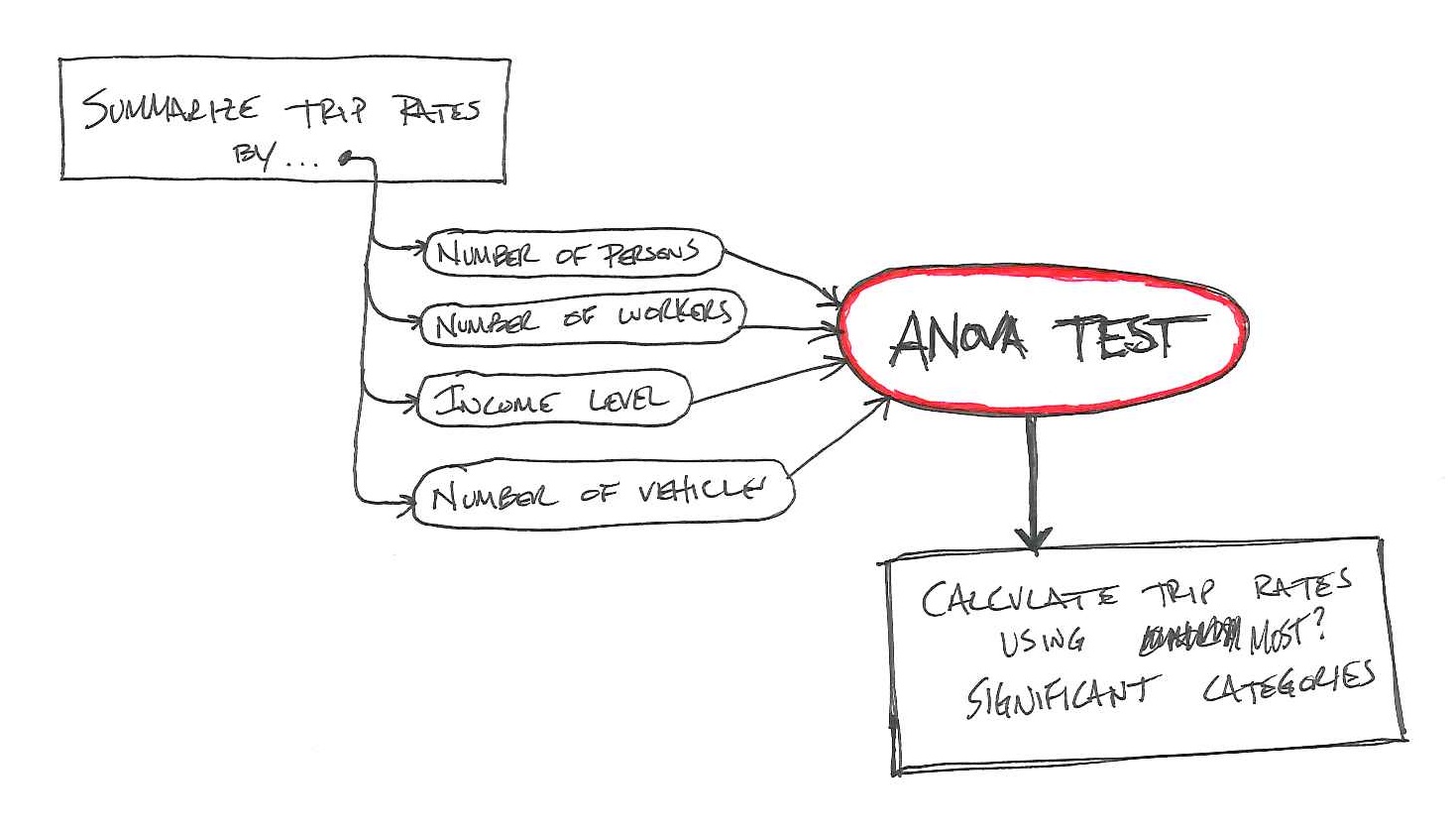
NCHRP Report 716 lays out a process that looks something like this when you make a graphic out of it:

So, the first part is to summarize the trips by persons, workers, income, and vehicles.  I’m going to skip income (I don’t care for using that as a variable).

This can be done pretty easily in R with a little bit of subsetting and ddply summaries that I’ve written about before. I split this into three groups based on area type, area type 1 is rural, 2 is suburban, and I combined 3 and 4 – urban and CBD.


hh.1<-subset(hhs,AreaType==1) hh.1.sumper<-ddply(hh.1,.(HHSize6),summarise,T.HBW=sum(HBW),T.HH=length(HHSize6),TR=T.HBW/T.HH) hh.1.sumwrk<-ddply(hh.1,.(Workers4),summarise,T.HBW=sum(HBW),T.HH=length(Workers4),TR=T.HBW/T.HH) hh.1.sumaut<-ddply(hh.1,.(HHVeh4),summarise,T.HBW=sum(HBW),T.HH=length(HHVeh4),TR=T.HBW/T.HH)

This makes three tables that looks like this:

>hh.1.sumper
HHSize6 T.HBW T.HH TR
1 1 9 54 0.1666667
2 2 77 98 0.7857143
3 3 24 38 0.6315789
4 4 36 40 0.9000000
5 5 18 10 1.8000000
6 6 4 6 0.6666667

Once all of this is performed (and it isn't much, as the code is very similar among three of the four lines above), you can analyze the variance:

#Perform analysis of variance, or ANOVA
> hh.1.perfit<-aov(TR~HHSize6,data=hh.1.sumper) > hh.1.wrkfit<-aov(TR~Workers4,data=hh.1.sumwrk) > hh.1.autfit<-aov(TR~HHVeh4,data=hh.1.sumaut) #Print summaries >summary(hh.1.perfit)
Df Sum Sq Mean Sq F value Pr(>F)
HHSize6 1 0.4824 0.4824 1.987 0.231
Residuals 4 0.9712 0.2428

> summary(hh.1.autfit)
Df Sum Sq Mean Sq F value Pr(>F)
HHVeh4 1 0.0994 0.09938 0.536 0.54
Residuals 2 0.3705 0.18526

The items above indicate that none of the three items above (persons per household, workers per household, or autos per household) are very significant predictors of home based work trips per household. Admittedly, I was a bit concerned here, but I pressed on to do the same for suburban and urban/CBD households and got something a little less concerning.

Suburban households

> summary(hh.2.autfit)
Df Sum Sq Mean Sq F value Pr(>F)
HHVeh4 1 0.6666 0.6666 23.05 0.0172 *
Residuals 3 0.0868 0.0289
---
Signif. codes: 0 ‘***’ 0.001 ‘**’ 0.01 ‘*’ 0.05 ‘.’ 0.1 ‘ ’ 1
> summary(hh.2.wrkfit)
Df Sum Sq Mean Sq F value Pr(>F)
Workers4 1 1.8951 1.8951 11.54 0.0425 *
Residuals 3 0.4926 0.1642
---
Signif. codes: 0 ‘***’ 0.001 ‘**’ 0.01 ‘*’ 0.05 ‘.’ 0.1 ‘ ’ 1
> summary(hh.2.perfit)
Df Sum Sq Mean Sq F value Pr(>F)
HHSize6 1 0.6530 0.6530 10.31 0.0326 *
Residuals 4 0.2534 0.0634
---
Signif. codes: 0 ‘***’ 0.001 ‘**’ 0.01 ‘*’ 0.05 ‘.’ 0.1 ‘ ’ 1

Urban and CBD Households

> summary(hh.34.autfit)
Df Sum Sq Mean Sq F value Pr(>F)
HHVeh4 1 1.8904 1.8904 32.8 0.0106 *
Residuals 3 0.1729 0.0576
---
Signif. codes: 0 ‘***’ 0.001 ‘**’ 0.01 ‘*’ 0.05 ‘.’ 0.1 ‘ ’ 1
> summary(hh.34.wrkfit)
Df Sum Sq Mean Sq F value Pr(>F)
Workers4 1 5.518 5.518 680 0.000124 ***
Residuals 3 0.024 0.008
---
Signif. codes: 0 ‘***’ 0.001 ‘**’ 0.01 ‘*’ 0.05 ‘.’ 0.1 ‘ ’ 1
> summary(hh.34.perfit)
Df Sum Sq Mean Sq F value Pr(>F)
HHSize6 1 0.7271 0.7271 9.644 0.036 *
Residuals 4 0.3016 0.0754
---
Signif. codes: 0 ‘***’ 0.001 ‘**’ 0.01 ‘*’ 0.05 ‘.’ 0.1 ‘ ’ 1


Another Way

Another way to do this is to do the ANOVA without summarizing the data. The results may not be the same or even support the same conclusion.

Rural

> summary(hh.1a.perfit)
Df Sum Sq Mean Sq F value Pr(>F)
HHSize6 1 15.3 15.310 10.61 0.00128 **
Residuals 244 352.0 1.442
---
Signif. codes: 0 ‘***’ 0.001 ‘**’ 0.01 ‘*’ 0.05 ‘.’ 0.1 ‘ ’ 1
> summary(hh.1a.wrkfit)
Df Sum Sq Mean Sq F value Pr(>F)
Workers4 1 60.46 60.46 48.08 3.64e-11 ***
Residuals 244 306.81 1.26
---
Signif. codes: 0 ‘***’ 0.001 ‘**’ 0.01 ‘*’ 0.05 ‘.’ 0.1 ‘ ’ 1
> summary(hh.1a.autfit)
Df Sum Sq Mean Sq F value Pr(>F)
HHVeh4 1 4.6 4.623 3.111 0.079 .
Residuals 244 362.6 1.486
---
Signif. codes: 0 ‘***’ 0.001 ‘**’ 0.01 ‘*’ 0.05 ‘.’ 0.1 ‘ ’ 1


Suburban

> hh.2a.perfit<-aov(HBW~HHSize6,data=hh.2) > hh.2a.wrkfit<-aov(HBW~Workers4,data=hh.2) > hh.2a.autfit<-aov(HBW~HHVeh4,data=hh.2) > summary(hh.2a.perfit)
Df Sum Sq Mean Sq F value Pr(>F)
HHSize6 1 136.1 136.05 101.9 <2e-16 *** Residuals 1160 1548.1 1.33 --- Signif. codes: 0 ‘***’ 0.001 ‘**’ 0.01 ‘*’ 0.05 ‘.’ 0.1 ‘ ’ 1 > summary(hh.2a.wrkfit)
Df Sum Sq Mean Sq F value Pr(>F)
Workers4 1 376.8 376.8 334.4 <2e-16 *** Residuals 1160 1307.3 1.1 --- Signif. codes: 0 ‘***’ 0.001 ‘**’ 0.01 ‘*’ 0.05 ‘.’ 0.1 ‘ ’ 1 > summary(hh.2a.autfit)
Df Sum Sq Mean Sq F value Pr(>F)
HHVeh4 1 103.2 103.20 75.72 <2e-16 *** Residuals 1160 1580.9 1.36 --- Signif. codes: 0 ‘***’ 0.001 ‘**’ 0.01 ‘*’ 0.05 ‘.’ 0.1 ‘ ’ 1
Urban/CBD

> hh.34a.perfit<-aov(HBW~HHSize6,data=hh.34) > hh.34a.wrkfit<-aov(HBW~Workers4,data=hh.34) > hh.34a.autfit<-aov(HBW~HHVeh4,data=hh.34) > summary(hh.34a.perfit)
Df Sum Sq Mean Sq F value Pr(>F)
HHSize6 1 77.1 77.07 64.38 4.93e-15 ***
Residuals 639 765.0 1.20
---
Signif. codes: 0 ‘***’ 0.001 ‘**’ 0.01 ‘*’ 0.05 ‘.’ 0.1 ‘ ’ 1
> summary(hh.34a.wrkfit)
Df Sum Sq Mean Sq F value Pr(>F)
Workers4 1 222.0 221.96 228.7 <2e-16 *** Residuals 639 620.1 0.97 --- Signif. codes: 0 ‘***’ 0.001 ‘**’ 0.01 ‘*’ 0.05 ‘.’ 0.1 ‘ ’ 1 > summary(hh.34a.autfit)
Df Sum Sq Mean Sq F value Pr(>F)
HHVeh4 1 91.1 91.12 77.53 <2e-16 *** Residuals 639 751.0 1.18 --- Signif. codes: 0 ‘***’ 0.001 ‘**’ 0.01 ‘*’ 0.05 ‘.’ 0.1 ‘ ’ 1

What this illustrates is that there is a difference between averages and raw numbers.

The next part of this will be to test a few different models to determine the actual trip rates to use, which will be the subject of the next blog post.

I’ve been doing a lot of statistical stuff over the past several weeks, and I think it is worth some value to the Interwebs if I try and post some of it.  I’m considering making it a course of some sort with some scrubbed HHTS data (no, I can’t post real peoples’ locations and names, I think I might get in a little bit of trouble for that).

The “syllabus” is roughly something like this (last update: 10 October 2013):

1. Intro to R: getting data in, making summaries
2. Trip rates – Linear and Non-linear modeling 6/7/13
3. Mode Choice Estimation in R 6/14/13
4. Trip rates – Averages 9/13/13
5. Complex Mode Choice Estimation in Biogeme <-Coming in two weeks or less!
6. Distribution Friction Factors
7. Distribution K Factors
8. Outputs and Graphics

I can’t guarantee that these will be the next eight weeks worth of posts – there will probably be some weeks with a different post, since I don’t know if I can get all this stuff done in six weeks, even with the head start I have.

In other news…

I’ve been disabling comments on these short posts that really don’t warrant any sort of responses.  I’ve been getting a lot of spam on this blog, so I’m cutting it down where I can.  This is not a global thing, I’ve been turning them off on certain posts, but the default is on.

Any statistical test that uses the t-distribution can be called a t-test. One of the most common is Student’s t-test, named after “Student,” the pseudonym that William Gosset used to hide his employment by the Guinness brewery in the early 1900s.  They didn’t want their competitors to know that they were making better beer with statistics.

From The Handbook of Biological Statistics.