I’ve been working through distribution in the model, and I was having a little bit of trouble.  As I looked into things, I found one place where QC is necessary to verify that things are working right.

The Logsums.

I didn’t like the shape of the curve from the friction factors I was getting, so I started looking into a variety of inputs to the mode choice model.  Like time and distance by car:

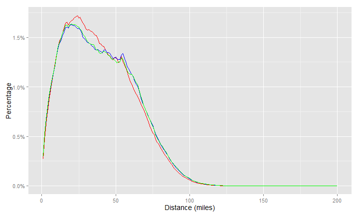
This is a comparison of distance. The red line is the new model, the blue and green are two different years of the old model.

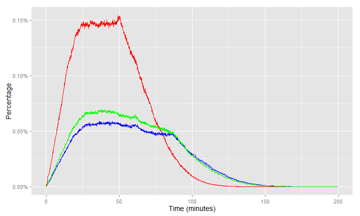
This is a comparison of zone-to-zone times. The red line is the new model, the blue and green are different years of the old model.

In both cases, these are as expected.  Since there are more (smaller) zones in the new model, there are more shorter times and distances.

The problem that crept up was the logsums coming from mode choice model for use in distribution:

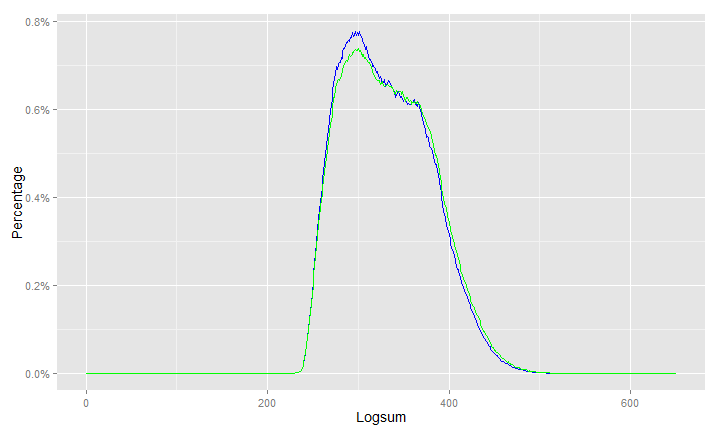
These are the logsums from the old model. Notice that the curve allows for some variation.

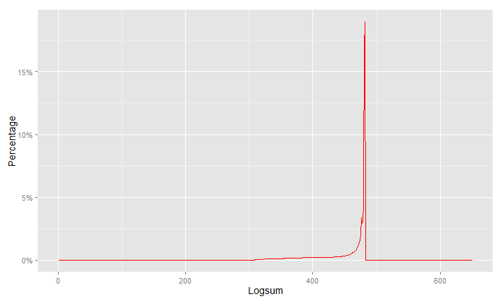
These are the logsums in the new model. This is a problem because of that ‘spike’.

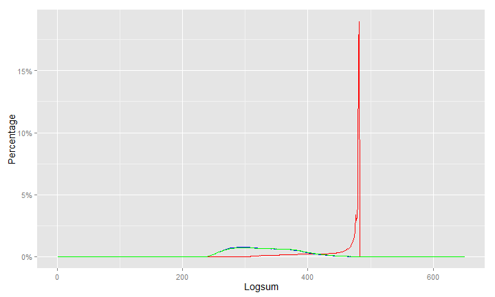
I put all the logsums on this, notice how the curve for the old model is dwarfed by the spike in the new model. This is bad.

So the question remains, what went wrong?

I believe the ultimate problem was that there was no limit on Bike and Pedestrian trips in the model, so it was generating some extreme values and somewhere and an infinity was happening in those modes causing the curve shown above.  I tested this by limiting the pedestrian trips to 5 miles (a fairly extreme value) and bike trips to 15 miles and re-running.  The logsums looked very different (again, the new model is the red line):

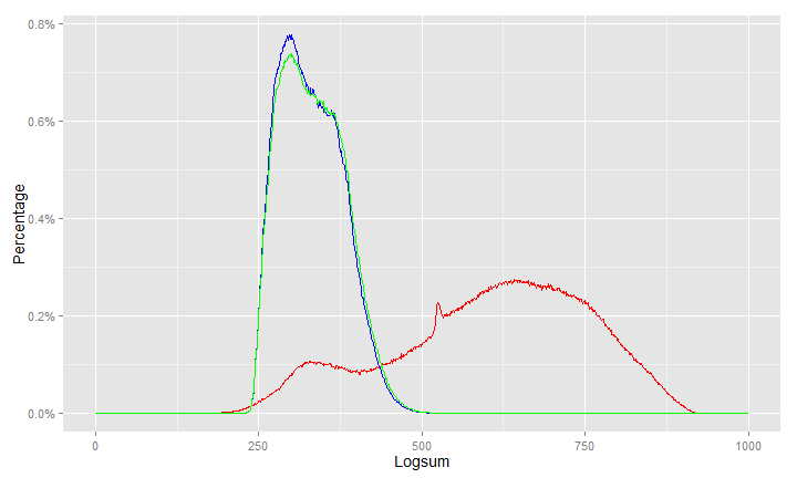
This is a comparison between the two model versions with fixed bicycle and pedestrian utility equations.

Note that the X axis range went from 650 (in the above plots) to 1000.  I’m not too concerned that the logsums in the new model have a larger range.  In fact, as long as those ranges are in the right place distribution may be better.  This is not final data, as I am still looking at a few other things to debug.

First note: I sent this to the support people at Citilabs recently, so maybe on the next update they’ll include this in the help document, as I think it is sorely missing.  Or maybe I’m just crazy (you kinda have to be crazy to do transportation modeling*) and have my own way of thinking.

In the OKI model, we have a nested logit mode choice structure that’s pretty common for MPOs our size – it’s had a history in several other MPOs.  The nesting structure looks like this:

The part that I think is missing in the Voyager Help File for XCHOICE is this:

XCHOICE ALTERNATIVES=LBW, LBP, LBK, EBW, EBP, EBK, LRW, LRP, LRK, WALK, BIKE, DA, SR2, SR3,
UTILITIESMW=141,142,143,144,145,146,147,148,149,110,111,112,113,114,
DEMANDMW=5,
ODEMANDMW=412,413,414,415,416,417,418,419,420,421,422,405,407,408,
SPLIT=LB 1 LBW 1 LBP 1 LBK,
SPLIT=EB 1 EBW 1 EBP 1 EBK,
SPLIT=LR 1 LRW 1 LRP 1 LRK,
SPLIT=TRAN 0.516 LB 0.516 EB 0.516 LR,
SPLIT=SR 1 SR2 1 SR3,
SPLIT=AUTO 0.516 SR 0.516 DA,
SPLIT=NONM 0.516 WALK 0.516 BIKE,
SPLIT=TOTAL 0.477 AUTO 0.477 TRAN 0.477 NONM,
SPLITCOMP=801,
STARTMW=900

More importantly, WHY this is important:

All those green, blue, red, and yellow marks are pointing things out – like what connects to what and so on.  Once these connections are made, you can get answers without a lot of effort.  It’s quite nice, really.  However, I haven’t figured out where to put upper-level coefficients, but in my latest estimation runs, those are out.

More Stuff

One of the more important things to get out of the mode choice model is the logsum values that would be used as the impedance for a gravity model distribution.  Once you have the above, it’s pretty easy.

First off, make your demand matrix have 100 trips per IJ pair:

MW[2]=100

Then, get the exponential of the SPLITCOMP matrix to get a usable logsum value.

MW[700]=EXP(MW[801])

Note that in the OKI model (and in other models that use walk access markets), this needs to be done multiple times and accumulated to another matrix:

MW[701]=MW[701]+(MW[5]*MW[700])

And then there is some post-processing that needs to be done at the end of the ILOOP:

JLOOP
IF(MW[2]>0)
MW[702]=MW[701]/MW[2] ;Denom
ELSE
MW[702]=0.00000000001
ENDIF

MW[704]=(LN(MW[702])/(COEFF[1]*CLSPRM*CLSSUB))+LOGADD
ENDJLOOP

704 is the output matrix.

—

* I have other forms of craziness, too.  I’ve recently announced – and made it “Facebook official” to my close friends and family – that I’m going to run a half marathon next spring.

This is second in the R in Transportation Modeling Series of posts.

I’ve been going between R, R Graphics Cookbook, NCHRP Report 716, and several other tasks, and finally got a chance to get back on actually performing the trip generation rates in the model.

The Process

NCHRP Report 716 lays out a process that looks something like this when you make a graphic out of it:

So, the first part is to summarize the trips by persons, workers, income, and vehicles.  I’m going to skip income (I don’t care for using that as a variable).

This can be done pretty easily in R with a little bit of subsetting and ddply summaries that I’ve written about before. I split this into three groups based on area type, area type 1 is rural, 2 is suburban, and I combined 3 and 4 – urban and CBD.


hh.1<-subset(hhs,AreaType==1) hh.1.sumper<-ddply(hh.1,.(HHSize6),summarise,T.HBW=sum(HBW),T.HH=length(HHSize6),TR=T.HBW/T.HH) hh.1.sumwrk<-ddply(hh.1,.(Workers4),summarise,T.HBW=sum(HBW),T.HH=length(Workers4),TR=T.HBW/T.HH) hh.1.sumaut<-ddply(hh.1,.(HHVeh4),summarise,T.HBW=sum(HBW),T.HH=length(HHVeh4),TR=T.HBW/T.HH)

This makes three tables that looks like this:

>hh.1.sumper
HHSize6 T.HBW T.HH TR
1 1 9 54 0.1666667
2 2 77 98 0.7857143
3 3 24 38 0.6315789
4 4 36 40 0.9000000
5 5 18 10 1.8000000
6 6 4 6 0.6666667

Once all of this is performed (and it isn't much, as the code is very similar among three of the four lines above), you can analyze the variance:

#Perform analysis of variance, or ANOVA
> hh.1.perfit<-aov(TR~HHSize6,data=hh.1.sumper) > hh.1.wrkfit<-aov(TR~Workers4,data=hh.1.sumwrk) > hh.1.autfit<-aov(TR~HHVeh4,data=hh.1.sumaut) #Print summaries >summary(hh.1.perfit)
Df Sum Sq Mean Sq F value Pr(>F)
HHSize6 1 0.4824 0.4824 1.987 0.231
Residuals 4 0.9712 0.2428

> summary(hh.1.autfit)
Df Sum Sq Mean Sq F value Pr(>F)
HHVeh4 1 0.0994 0.09938 0.536 0.54
Residuals 2 0.3705 0.18526

The items above indicate that none of the three items above (persons per household, workers per household, or autos per household) are very significant predictors of home based work trips per household. Admittedly, I was a bit concerned here, but I pressed on to do the same for suburban and urban/CBD households and got something a little less concerning.

Suburban households

> summary(hh.2.autfit)
Df Sum Sq Mean Sq F value Pr(>F)
HHVeh4 1 0.6666 0.6666 23.05 0.0172 *
Residuals 3 0.0868 0.0289
---
Signif. codes: 0 ‘***’ 0.001 ‘**’ 0.01 ‘*’ 0.05 ‘.’ 0.1 ‘ ’ 1
> summary(hh.2.wrkfit)
Df Sum Sq Mean Sq F value Pr(>F)
Workers4 1 1.8951 1.8951 11.54 0.0425 *
Residuals 3 0.4926 0.1642
---
Signif. codes: 0 ‘***’ 0.001 ‘**’ 0.01 ‘*’ 0.05 ‘.’ 0.1 ‘ ’ 1
> summary(hh.2.perfit)
Df Sum Sq Mean Sq F value Pr(>F)
HHSize6 1 0.6530 0.6530 10.31 0.0326 *
Residuals 4 0.2534 0.0634
---
Signif. codes: 0 ‘***’ 0.001 ‘**’ 0.01 ‘*’ 0.05 ‘.’ 0.1 ‘ ’ 1

Urban and CBD Households

> summary(hh.34.autfit)
Df Sum Sq Mean Sq F value Pr(>F)
HHVeh4 1 1.8904 1.8904 32.8 0.0106 *
Residuals 3 0.1729 0.0576
---
Signif. codes: 0 ‘***’ 0.001 ‘**’ 0.01 ‘*’ 0.05 ‘.’ 0.1 ‘ ’ 1
> summary(hh.34.wrkfit)
Df Sum Sq Mean Sq F value Pr(>F)
Workers4 1 5.518 5.518 680 0.000124 ***
Residuals 3 0.024 0.008
---
Signif. codes: 0 ‘***’ 0.001 ‘**’ 0.01 ‘*’ 0.05 ‘.’ 0.1 ‘ ’ 1
> summary(hh.34.perfit)
Df Sum Sq Mean Sq F value Pr(>F)
HHSize6 1 0.7271 0.7271 9.644 0.036 *
Residuals 4 0.3016 0.0754
---
Signif. codes: 0 ‘***’ 0.001 ‘**’ 0.01 ‘*’ 0.05 ‘.’ 0.1 ‘ ’ 1


Another Way

Another way to do this is to do the ANOVA without summarizing the data. The results may not be the same or even support the same conclusion.

Rural

> summary(hh.1a.perfit)
Df Sum Sq Mean Sq F value Pr(>F)
HHSize6 1 15.3 15.310 10.61 0.00128 **
Residuals 244 352.0 1.442
---
Signif. codes: 0 ‘***’ 0.001 ‘**’ 0.01 ‘*’ 0.05 ‘.’ 0.1 ‘ ’ 1
> summary(hh.1a.wrkfit)
Df Sum Sq Mean Sq F value Pr(>F)
Workers4 1 60.46 60.46 48.08 3.64e-11 ***
Residuals 244 306.81 1.26
---
Signif. codes: 0 ‘***’ 0.001 ‘**’ 0.01 ‘*’ 0.05 ‘.’ 0.1 ‘ ’ 1
> summary(hh.1a.autfit)
Df Sum Sq Mean Sq F value Pr(>F)
HHVeh4 1 4.6 4.623 3.111 0.079 .
Residuals 244 362.6 1.486
---
Signif. codes: 0 ‘***’ 0.001 ‘**’ 0.01 ‘*’ 0.05 ‘.’ 0.1 ‘ ’ 1


Suburban

> hh.2a.perfit<-aov(HBW~HHSize6,data=hh.2) > hh.2a.wrkfit<-aov(HBW~Workers4,data=hh.2) > hh.2a.autfit<-aov(HBW~HHVeh4,data=hh.2) > summary(hh.2a.perfit)
Df Sum Sq Mean Sq F value Pr(>F)
HHSize6 1 136.1 136.05 101.9 <2e-16 *** Residuals 1160 1548.1 1.33 --- Signif. codes: 0 ‘***’ 0.001 ‘**’ 0.01 ‘*’ 0.05 ‘.’ 0.1 ‘ ’ 1 > summary(hh.2a.wrkfit)
Df Sum Sq Mean Sq F value Pr(>F)
Workers4 1 376.8 376.8 334.4 <2e-16 *** Residuals 1160 1307.3 1.1 --- Signif. codes: 0 ‘***’ 0.001 ‘**’ 0.01 ‘*’ 0.05 ‘.’ 0.1 ‘ ’ 1 > summary(hh.2a.autfit)
Df Sum Sq Mean Sq F value Pr(>F)
HHVeh4 1 103.2 103.20 75.72 <2e-16 *** Residuals 1160 1580.9 1.36 --- Signif. codes: 0 ‘***’ 0.001 ‘**’ 0.01 ‘*’ 0.05 ‘.’ 0.1 ‘ ’ 1
Urban/CBD

> hh.34a.perfit<-aov(HBW~HHSize6,data=hh.34) > hh.34a.wrkfit<-aov(HBW~Workers4,data=hh.34) > hh.34a.autfit<-aov(HBW~HHVeh4,data=hh.34) > summary(hh.34a.perfit)
Df Sum Sq Mean Sq F value Pr(>F)
HHSize6 1 77.1 77.07 64.38 4.93e-15 ***
Residuals 639 765.0 1.20
---
Signif. codes: 0 ‘***’ 0.001 ‘**’ 0.01 ‘*’ 0.05 ‘.’ 0.1 ‘ ’ 1
> summary(hh.34a.wrkfit)
Df Sum Sq Mean Sq F value Pr(>F)
Workers4 1 222.0 221.96 228.7 <2e-16 *** Residuals 639 620.1 0.97 --- Signif. codes: 0 ‘***’ 0.001 ‘**’ 0.01 ‘*’ 0.05 ‘.’ 0.1 ‘ ’ 1 > summary(hh.34a.autfit)
Df Sum Sq Mean Sq F value Pr(>F)
HHVeh4 1 91.1 91.12 77.53 <2e-16 *** Residuals 639 751.0 1.18 --- Signif. codes: 0 ‘***’ 0.001 ‘**’ 0.01 ‘*’ 0.05 ‘.’ 0.1 ‘ ’ 1

What this illustrates is that there is a difference between averages and raw numbers.

The next part of this will be to test a few different models to determine the actual trip rates to use, which will be the subject of the next blog post.

One thing that can drastically speed Cube is using a DLL to do big tasks, like Nested Logit Mode Choice. However, doing this can be fraught with hair-pulling errors.  This post shows some techniques to keep your hair on your head.  This post is written for a travel demand modeler, not a computer science person!

RTFM (Read The Fine Manual)

Read the help file for Matrix CALL statement.  The struct statement is pretty important, and the sprintf lines will be used throughout.

Memory Pointers

One of the most important things to understand is that because there are so many variables that can be passed between Cube and the C++ DLL, the memory pointers are passed instead.  Also, one of those “pull your hair out” things relates to this – if you attempt to access a memory pointer that hasn’t been initialized, you get a crash that gives no error.

Because of this, the variables in the struct statement have a *, which notes that it is a memory pointer.

To keep from getting the crash-with-no-error, the following statement works well to test and allows a default to be used if the variable ‘MarketSegments’ is not set in Cube.

int MarketSegments=4;

if(Stack->pfFindVar("MarketSegments")!=0)
MarketSegments=(int)*Stack->pfFindVar("MarketSegments");

Matrix In, Matrix Out

While the Help file says that you can get to defined working matrixes using

static double **MW;
MW=(*Stack->pfFindVar)("MW",1);

I can’t get it to work using C++ (I have gotten it to work in C).  Instead, use the following:

static double **MW=NULL;
MW=Stack->MW;

This will enable you to use MW[m][j] (where m is the MW number, and j is the j-zone).

You can also set the MW variables, but it does NOTHING if you don’t set the MW to something in Cube Voyager.  Ergo, if you set

MW[101][j]=10;

Your output will be 0 unless you do the following in Cube Voyager

MW[101]=0
CALL...

Array Variables

One of the tricks I use to get array variables out of Cube is this

float ArrayVariable[7]={0,0,0,0,0,0,0};  //Note: I'm using 1-6.  Setting this to 7 means 0-6.  Setting it to 6 would mean 0-5
if(Stack->pfFindVar("ArrayVariable")>0){
double* tmpAV=NULL;
tmpAV=Stack->pfFindVar("ArrayVariable",1,2,3,4,5,6);
for(int x=1;x<=6;x++)
ArrayVariable[x]=tmpAV[x];
}

This code above checks that the ArrayVariable, fills them into a temporary variable, and then sets the actual variable.

Compilation Linker Settings

When compiling, you need to set the EXPORT flag so the name is predictable and correct.  To do this, go to your project’s property pages – Configuration Properties – Linker – Command Line.  You need to add “/EXPORT:FunctionName” under Additional Options.  See the screenshot below

.

Other Weird Stuff

Any error in C++ that does not cause a compilation error results in one of those useless “this program has an error and will be closed” and crashes Task Monitor.  That being said, write messages to the output file frequently (if at least during debugging).  This can assist with finding typos (like, say, %10.65f in an sprintf statement, which means 65 decimal places in a 10-width line).

Credit for this goes to Citilabs Support, although I made some adaptations.

In Matrix when using DBI, PAR ZONES=1 will effectively shut off Cluster. Therefore, the following works really well.


DISTRIBUTEINTRASTEP ProcessID=Cluster ProcessList={CORES}

LOOP _r=start,end
x=DBIReadRecord(1,_r)
ENDLOOP


This script sets each core to process an equal portion of the database with any remainder (e.g if you cluster 4 records over 3 cores) to the last core.

There are several issues with long travel demand model run times.  Deep down, these are supposed to be planning tools, and taking too long for results can reduce the practicality of using a travel demand model in decision making.

In Cube Voyager, I’ve been finding more ways to cut runtimes down as much as possible, and below is the list with some of the rationale.

Keep JLoops at a Minimum

The Matrix program runs in an implied ILOOP.  This being the case, anything in the script runs many times (as many as the zones you have).  Using a JLOOP in a 2,000 zone model means that there are  4,000,000 calculations to be done for each COMP statement.  What happens if you have 3 COMP statements?  You go from 4,000,000 to 12,000,000 calculations.  This is even worse if the calculations include a lookup function, which are generally slow.

Keep Files Small – Only Write What You Have To

This is a no-brainer.  The more that Cube (or anything, for that matter) has to write to disk, the longer the runtime.

Replace RECI with DBI wherever possible

DBI can be clustered (look for a post on that in the coming weeks).  While I’m not sure if there is any difference on one core, being able to use Cluster is the trump card.

Use Cluster Dynamically and Wherever Possible

Standardize the Cluster ID in your code, but set the process list to a catalog key as with below:

DISTRIBUTEINTRASTEP CLUSTERID=Cluster PROCESSLIST=2-{CORES}

Using Cluster to your advantage is critical to having a fast model.

It occurred to me that many people likely do not understand all of the terminology of travel demand models.  Because of this, I felt the need to list many of them here. Read the rest of this post… »

The center of most travel demand models is the “Four Step Model”.  This model was created in the 1950s to determine the demand on roadways.  The four steps include:

1. Trip Generation
2. Trip Distribution
3. Mode Choice
4. Trip Assignment

Read the rest of this post… »