During the peer review, one thing that we were told to look at was the variance in the cells of our cross-classification table.

Like all statistics, variance needs to be looked at in context with other statistics.  To illustrate this, I created some fake data In Excel.

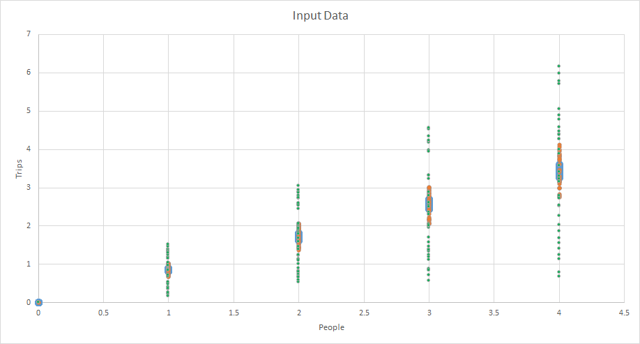
This is what the data looks like. It is all random and perfect, but you can see that some is “tighter” than others.

The first thing I looked at was the variance compared to the mean.

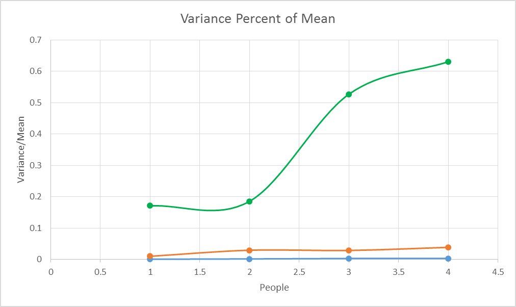
This is the variance compared to the mean. Note that the colors are the same as on the input sheet. The green line (which had the largest random scatter component) is way high compared to the other two, which are much more centralized around the mean.

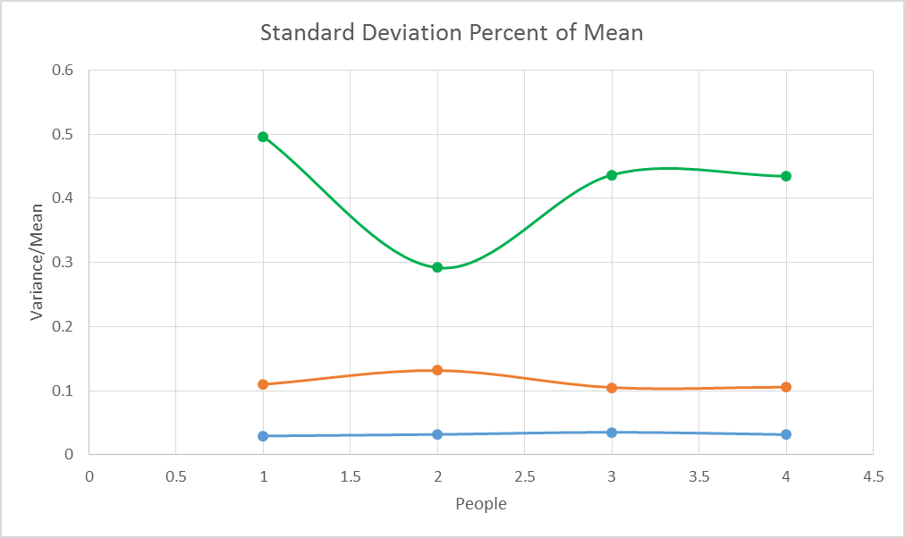
I looked at the standard deviation as well, but variance looks better to me.

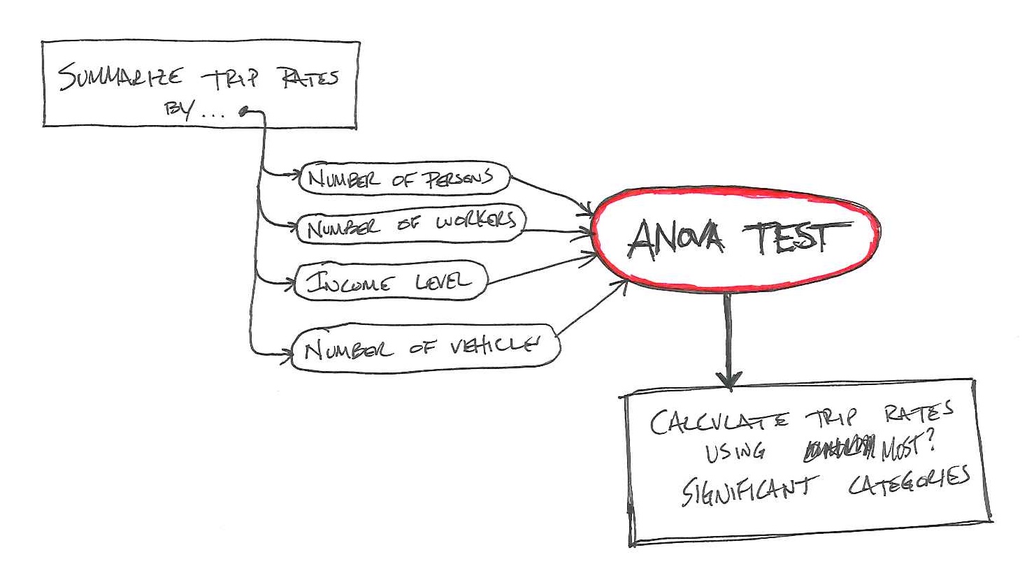
What does this mean?  Well, lets take a look at it using a subset of NHTS 2009 data.

I looked at the average trips per household by number of workers, and the table below lists the average by worker.

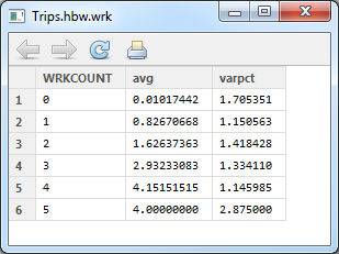
The var/mean (the varpct column in the table) is pretty high.  The correlation isn’t bad at 0.616.  However, there are 3,143 observed trips in the table, and this method results in the same number of trips.

Next, I looked at average trips per household by workers and income.

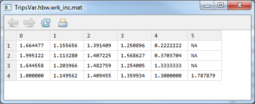
Variance/mean of trips

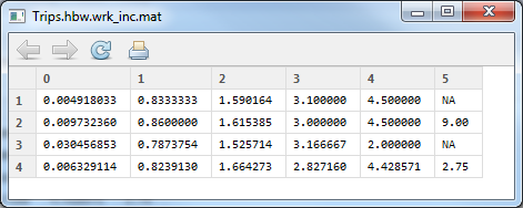
Average Trip Rates by HH

They’re a little better looking.  The correlation is 0.623, so that’s a little better, and the total trips is 3,143.  Yes, that is the exact number of trips in the table.  Looking at the sum of the difference (which in this case should be zero), it came up to -5.432×10^-14… that’s quite close to zero!

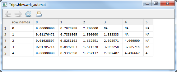
Mean trips per household by workers and autos (rows are autos, columns are workers)

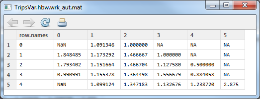
Variance/mean trips per household by workers and autos (rows are autos, columns are workers)

By workers and autos was similar – the correlation was 0.619, and the total trips is 3,143.  Since it was the exact same number as the last time, I checked the difference in the same manner, and found that the total difference was 4.14×10^-14.  Different by a HUGE (not!) amount.

Summary

There are a few things to look at.

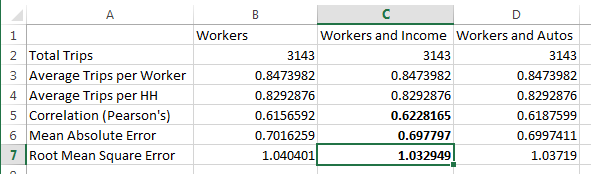
Summary of various factors.

Ultimately, this wasn’t as different as I hoped to show.  I was hoping to show some bad data vs. good data from the NHTS, but without intentionally monkeying with the data, it was hard to get something better.

-A-

This is second in the R in Transportation Modeling Series of posts.

I’ve been going between R, R Graphics Cookbook, NCHRP Report 716, and several other tasks, and finally got a chance to get back on actually performing the trip generation rates in the model.

The Process

NCHRP Report 716 lays out a process that looks something like this when you make a graphic out of it:

So, the first part is to summarize the trips by persons, workers, income, and vehicles.  I’m going to skip income (I don’t care for using that as a variable).

This can be done pretty easily in R with a little bit of subsetting and ddply summaries that I’ve written about before. I split this into three groups based on area type, area type 1 is rural, 2 is suburban, and I combined 3 and 4 – urban and CBD.


hh.1<-subset(hhs,AreaType==1) hh.1.sumper<-ddply(hh.1,.(HHSize6),summarise,T.HBW=sum(HBW),T.HH=length(HHSize6),TR=T.HBW/T.HH) hh.1.sumwrk<-ddply(hh.1,.(Workers4),summarise,T.HBW=sum(HBW),T.HH=length(Workers4),TR=T.HBW/T.HH) hh.1.sumaut<-ddply(hh.1,.(HHVeh4),summarise,T.HBW=sum(HBW),T.HH=length(HHVeh4),TR=T.HBW/T.HH)

This makes three tables that looks like this:

>hh.1.sumper
HHSize6 T.HBW T.HH TR
1 1 9 54 0.1666667
2 2 77 98 0.7857143
3 3 24 38 0.6315789
4 4 36 40 0.9000000
5 5 18 10 1.8000000
6 6 4 6 0.6666667

Once all of this is performed (and it isn't much, as the code is very similar among three of the four lines above), you can analyze the variance:

#Perform analysis of variance, or ANOVA
> hh.1.perfit<-aov(TR~HHSize6,data=hh.1.sumper) > hh.1.wrkfit<-aov(TR~Workers4,data=hh.1.sumwrk) > hh.1.autfit<-aov(TR~HHVeh4,data=hh.1.sumaut) #Print summaries >summary(hh.1.perfit)
Df Sum Sq Mean Sq F value Pr(>F)
HHSize6 1 0.4824 0.4824 1.987 0.231
Residuals 4 0.9712 0.2428

> summary(hh.1.autfit)
Df Sum Sq Mean Sq F value Pr(>F)
HHVeh4 1 0.0994 0.09938 0.536 0.54
Residuals 2 0.3705 0.18526

The items above indicate that none of the three items above (persons per household, workers per household, or autos per household) are very significant predictors of home based work trips per household. Admittedly, I was a bit concerned here, but I pressed on to do the same for suburban and urban/CBD households and got something a little less concerning.

Suburban households

> summary(hh.2.autfit)
Df Sum Sq Mean Sq F value Pr(>F)
HHVeh4 1 0.6666 0.6666 23.05 0.0172 *
Residuals 3 0.0868 0.0289
---
Signif. codes: 0 ‘***’ 0.001 ‘**’ 0.01 ‘*’ 0.05 ‘.’ 0.1 ‘ ’ 1
> summary(hh.2.wrkfit)
Df Sum Sq Mean Sq F value Pr(>F)
Workers4 1 1.8951 1.8951 11.54 0.0425 *
Residuals 3 0.4926 0.1642
---
Signif. codes: 0 ‘***’ 0.001 ‘**’ 0.01 ‘*’ 0.05 ‘.’ 0.1 ‘ ’ 1
> summary(hh.2.perfit)
Df Sum Sq Mean Sq F value Pr(>F)
HHSize6 1 0.6530 0.6530 10.31 0.0326 *
Residuals 4 0.2534 0.0634
---
Signif. codes: 0 ‘***’ 0.001 ‘**’ 0.01 ‘*’ 0.05 ‘.’ 0.1 ‘ ’ 1

Urban and CBD Households

> summary(hh.34.autfit)
Df Sum Sq Mean Sq F value Pr(>F)
HHVeh4 1 1.8904 1.8904 32.8 0.0106 *
Residuals 3 0.1729 0.0576
---
Signif. codes: 0 ‘***’ 0.001 ‘**’ 0.01 ‘*’ 0.05 ‘.’ 0.1 ‘ ’ 1
> summary(hh.34.wrkfit)
Df Sum Sq Mean Sq F value Pr(>F)
Workers4 1 5.518 5.518 680 0.000124 ***
Residuals 3 0.024 0.008
---
Signif. codes: 0 ‘***’ 0.001 ‘**’ 0.01 ‘*’ 0.05 ‘.’ 0.1 ‘ ’ 1
> summary(hh.34.perfit)
Df Sum Sq Mean Sq F value Pr(>F)
HHSize6 1 0.7271 0.7271 9.644 0.036 *
Residuals 4 0.3016 0.0754
---
Signif. codes: 0 ‘***’ 0.001 ‘**’ 0.01 ‘*’ 0.05 ‘.’ 0.1 ‘ ’ 1


Another Way

Another way to do this is to do the ANOVA without summarizing the data. The results may not be the same or even support the same conclusion.

Rural

> summary(hh.1a.perfit)
Df Sum Sq Mean Sq F value Pr(>F)
HHSize6 1 15.3 15.310 10.61 0.00128 **
Residuals 244 352.0 1.442
---
Signif. codes: 0 ‘***’ 0.001 ‘**’ 0.01 ‘*’ 0.05 ‘.’ 0.1 ‘ ’ 1
> summary(hh.1a.wrkfit)
Df Sum Sq Mean Sq F value Pr(>F)
Workers4 1 60.46 60.46 48.08 3.64e-11 ***
Residuals 244 306.81 1.26
---
Signif. codes: 0 ‘***’ 0.001 ‘**’ 0.01 ‘*’ 0.05 ‘.’ 0.1 ‘ ’ 1
> summary(hh.1a.autfit)
Df Sum Sq Mean Sq F value Pr(>F)
HHVeh4 1 4.6 4.623 3.111 0.079 .
Residuals 244 362.6 1.486
---
Signif. codes: 0 ‘***’ 0.001 ‘**’ 0.01 ‘*’ 0.05 ‘.’ 0.1 ‘ ’ 1


Suburban

> hh.2a.perfit<-aov(HBW~HHSize6,data=hh.2) > hh.2a.wrkfit<-aov(HBW~Workers4,data=hh.2) > hh.2a.autfit<-aov(HBW~HHVeh4,data=hh.2) > summary(hh.2a.perfit)
Df Sum Sq Mean Sq F value Pr(>F)
HHSize6 1 136.1 136.05 101.9 <2e-16 *** Residuals 1160 1548.1 1.33 --- Signif. codes: 0 ‘***’ 0.001 ‘**’ 0.01 ‘*’ 0.05 ‘.’ 0.1 ‘ ’ 1 > summary(hh.2a.wrkfit)
Df Sum Sq Mean Sq F value Pr(>F)
Workers4 1 376.8 376.8 334.4 <2e-16 *** Residuals 1160 1307.3 1.1 --- Signif. codes: 0 ‘***’ 0.001 ‘**’ 0.01 ‘*’ 0.05 ‘.’ 0.1 ‘ ’ 1 > summary(hh.2a.autfit)
Df Sum Sq Mean Sq F value Pr(>F)
HHVeh4 1 103.2 103.20 75.72 <2e-16 *** Residuals 1160 1580.9 1.36 --- Signif. codes: 0 ‘***’ 0.001 ‘**’ 0.01 ‘*’ 0.05 ‘.’ 0.1 ‘ ’ 1
Urban/CBD

> hh.34a.perfit<-aov(HBW~HHSize6,data=hh.34) > hh.34a.wrkfit<-aov(HBW~Workers4,data=hh.34) > hh.34a.autfit<-aov(HBW~HHVeh4,data=hh.34) > summary(hh.34a.perfit)
Df Sum Sq Mean Sq F value Pr(>F)
HHSize6 1 77.1 77.07 64.38 4.93e-15 ***
Residuals 639 765.0 1.20
---
Signif. codes: 0 ‘***’ 0.001 ‘**’ 0.01 ‘*’ 0.05 ‘.’ 0.1 ‘ ’ 1
> summary(hh.34a.wrkfit)
Df Sum Sq Mean Sq F value Pr(>F)
Workers4 1 222.0 221.96 228.7 <2e-16 *** Residuals 639 620.1 0.97 --- Signif. codes: 0 ‘***’ 0.001 ‘**’ 0.01 ‘*’ 0.05 ‘.’ 0.1 ‘ ’ 1 > summary(hh.34a.autfit)
Df Sum Sq Mean Sq F value Pr(>F)
HHVeh4 1 91.1 91.12 77.53 <2e-16 *** Residuals 639 751.0 1.18 --- Signif. codes: 0 ‘***’ 0.001 ‘**’ 0.01 ‘*’ 0.05 ‘.’ 0.1 ‘ ’ 1

What this illustrates is that there is a difference between averages and raw numbers.

The next part of this will be to test a few different models to determine the actual trip rates to use, which will be the subject of the next blog post.

This post will talk about building linear and non-linear models of trip rates in R.  If you haven’t read the first part of this series, please do so, partly because this builds on it.

Simple Linear Models

Simple linear models are, well, simple in R.  An example of a fairly easy linear model with two factors is:

inTab.hbsh

This creates a simple linear home-based-shopping trip generation model based on workers and household size.  Once the estimation completes (it should take less than a second), the summary should show the following data:

> summary(hbsh.lm.W_H)

Call:

lm(formula = N ~ Workers4 + HHSize6, data = hbsh)

Residuals:

    Min      1Q  Median      3Q     Max 

-2.2434 -1.1896 -0.2749  0.7251 11.2946 

Coefficients:

            Estimate Std. Error t value Pr(>|t|)    

(Intercept)  1.79064    0.10409  17.203  < 2e-16 ***

Workers4    -0.02690    0.05848  -0.460    0.646    

HHSize6      0.24213    0.04365   5.547 3.58e-08 ***

---

Signif. codes:  0 ‘***’ 0.001 ‘**’ 0.01 ‘*’ 0.05 ‘.’ 0.1 ‘ ’ 1 

Residual standard error: 1.649 on 1196 degrees of freedom

Multiple R-squared: 0.03228,    Adjusted R-squared: 0.03066 

F-statistic: 19.95 on 2 and 1196 DF,  p-value: 3.008e-09

What all this means is:

Trips = -0.0269*workers+0.24213*HHSize+1.79064

The important things to note on this is that the intercept is very significant (that's bad) and the R2 is 0.03066 (that's horrible).  There's more here, but it's more details.

Non-Linear Least Squares

When doing a non-linear model, the nls function is the way to go.  The two lines below create a trips data frame, and then run a non-linear least-squares model estimation on it (note that the first line is long and wraps to the second line).

trips=3),

start=c(a=1,b=1),trace=true)

The second line does the actual non-linear least-squares estimation.  The input formula is T=a*e^(HHSize+b).  In this type of model, starting values for a and b have to be given to the model.

The summary of this model is a little different:

> summary( trips.hbo.nls.at3p)

Formula: T.HBO ~ a * log(HHSize6 + b)

Parameters:

  Estimate Std. Error t value Pr(>|t|)    

a   1.8672     0.1692  11.034  < 2e-16 ***

b   1.2366     0.2905   4.257 2.58e-05 ***

---

Signif. codes:  0 ‘***’ 0.001 ‘**’ 0.01 ‘*’ 0.05 ‘.’ 0.1 ‘ ’ 1 

Residual standard error: 2.095 on 402 degrees of freedom

Number of iterations to convergence: 4 

Achieved convergence tolerance: 1.476e-07 

It doesn't perform R2 on this because it can't directly.  However, we can because we know the actual values and the model predicts the values.  So, one thing that can be done is a plot:

> plot(c(0,10),c(0,10),type='l',xlab='Observed Trips',ylab='Predicted Trips')

> points(subset(trips,AreaType>=3)$T.HBO,fitted(trips.hbo.nls.at3p),col='red')

The resulting graph looks like this.  Not particularly good, but there is also no scale as to the frequency along the 45° line.

R2 is still a good measure here.  There's probably an easier way to do this, but this way is pretty simple.  

testTable=3)$T.HBO,fitted(trips.hbo.nls.at3p)))

cor(testTable$X1,testTable$X2)

Since I didn't correct the column names when I created the data frame, R used X1 and X2, as evidenced by checking the summary of testTable:

> summary(testTable)

       X1               X2       

 Min.   : 0.000   Min.   :1.503  

 1st Qu.: 1.000   1st Qu.:1.503  

 Median : 2.000   Median :2.193  

 Mean   : 2.072   Mean   :2.070  

 3rd Qu.: 3.000   3rd Qu.:2.193  

 Max.   :23.000   Max.   :3.696  

So the R2 value is pretty bad...

> cor(testTable$X1,testTable$X2)

[1] 0.2755101

It's better than some of the others, after all, this is semirandom human behavior.

That's it for now.  My next post will be... MORE R!

Also, I have a quick shout-out to Jeremy Raw at FHWA for help via email related to this.  He helped me through some issues via email, and parts of his email helped parts of this post.

One thing that is constantly bounced around is why tour-based modeling is better than trip based modeling.  We’ve been using trip based modeling for 50 years, isn’t it timeless?

No.

Fifty years ago, when the trip based modeling methodologies were developed, the primary reason was to evaluate highway improvements.  While tolling was in use, the bonding requirements were likely different.  Transit, while extremely important, was not in the public realm (the streetcars were normally privately owned by the area’s electric company).

Now, there are a lot of demands on travel models:

• Tolling/Toll Road analysis at a better level
• Different tolling schemes (area tolling, cordon tolling)
• Travel Demand Management (telecommuting, flex hours, flex time, alternative schedules)
• Better freight modeling (which now is becoming commodity flow and commercial vehicle modeling)
• Varying levels of transit (local bus, express bus, intercity bus, BRT, light rail, and commuter rail

While many of these can be done with trip based models, most of them cannot be done well with trip based models.  There are a number of reasons, but the few that come to mind are aggregation bias, modal inconsistency, and household interrelationships.

Aggregation Bias

Aggregation bias occurs when averages are used to determine an outcome.  For example, using a zonal average vehicles per household, you miss the components that form the average, such as:

20 households, average VPHH = 2.2
2 HH VPHH = 0
5 HH VPHH = 1
4 HH VPHH = 2
6 HH VPHH = 3
3 HH VPHH = 4+

The trip generation and modal choices (car, bus, bike, walk, etc.) among these households are all different, and are even more more different if you look at the number of workers per household.

Modal Inconsistency

In trip based modeling, “people” are not tracked throughout their day.  So, if someone rides the bus to work, there is nothing in the model to ensure that they don’t drive from work to get lunch.  While we don’t want to force people to use the same mode, since many people will use the bus to get to work and then walk to lunch or to go shopping during lunch, we want to make sure that there is some compatibility of modes.

Household Interrelationships

One of the features of of tour based models is determining each person’s daily activity pattern.  During this process, certain person types can determine what another person is doing.  For example, if a preschool age child is staying home, an adult (whether they are a worker or not) HAS to stay home.  Another example is if a school-non-driving-age child is going on a non-mandatory trip, an adult must accompany them.  Trip based models don’t know about the household makeup and the household interaction.

The above are only three of the many reasons why tour-based modeling is important.  There are many more, but I feel these are some of the most important and some of the easiest to understand.

Trip generation is likely one of the easiest parts of the four step process.  Normally, the most difficult part of dealing with trip generation is getting the input socioeconomic (population and employment) data correct.  This post explains how trip generation is calculated in the model… Read the rest of this post… »