It’s not Thanksgiving, it’s ITM.

I figured that since nothing has really been making it to the blog lately (that will change starting now!), I should mention my way getting from Cincinnati (CVG) to Baltimore (BWI) and back.
First off, the flights from Cincinnati have been horrible ever since Delta decided to functionally de-hub the airport.  It seems I’m always making compromises for my DC trips, and the flights from CVG to BWI are late in the day arriving after 5:00 PM.  The workshops on Sunday were at 1:00 PM, and there were things I didn’t want to miss.
Being the problem solver I am, I looked into other options.  I figured out something, and I’m writing this the day before I leave and thinking “nothing can possibly go wrong here, right?”.  The day-of-travel additions will be in italics.  Or pictures.
Automobiles: Leg 1Â -Â Home to Airport
This is the most control I’ll have today. Â I drive my little red S-10 to the parking lot across the freeway from the airport and take their shuttle from the lot to the arrivals area. Â I’ve used this service (Cincinnati Fast Park & Relax) dozens of times without issues. Â They rock. Â God, I hope they’re awake at 4:30 AM!!!
They were awake and I got a pretty good parking spot near the front!
Planes: Leg 2 – CVG to Washington Reagan International
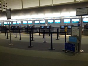
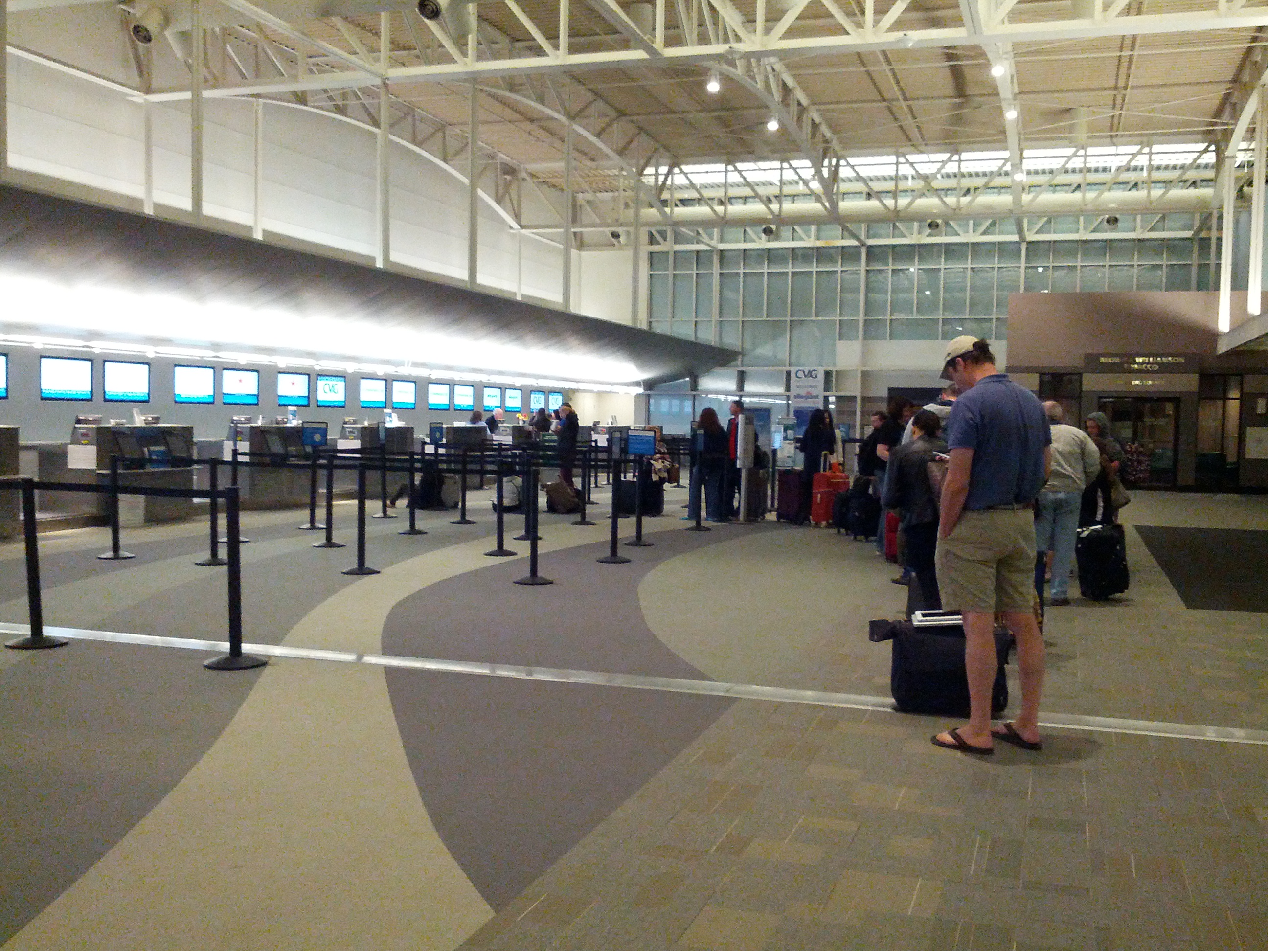
That is correct.  Flights from CVG to DCA are extraordinarily early (and dear reader, as you read the rest you’ll see why this is critically important).  This is a US Airways flight.  I learned recently (for the TRB Annual Meeting in January) to print my boarding pass early and fit everything into a carry-on.  Since they are now owned by Unamerican Airlines their baggage counter will have a line stretching out to downtown Cincinnati (about the distance of a half marathon!) while every other airline has few people in line and FAR BETTER SERVICE.
Thank God I printed my boarding pass in advance. Â This was the line at the US Airways check-in counter. Â I realized after my last trip to the TRB Annual Meeting in Washington that pre-paying for checked baggage is of no help. Â In fact, I think some of these people were in line since last January. Â US Airways sucks, especially now that they are part of American Airlines, which is the WORST airline I have ever flown. Â

The front of the line has been there since January 12, 2014. I’m sure of it.
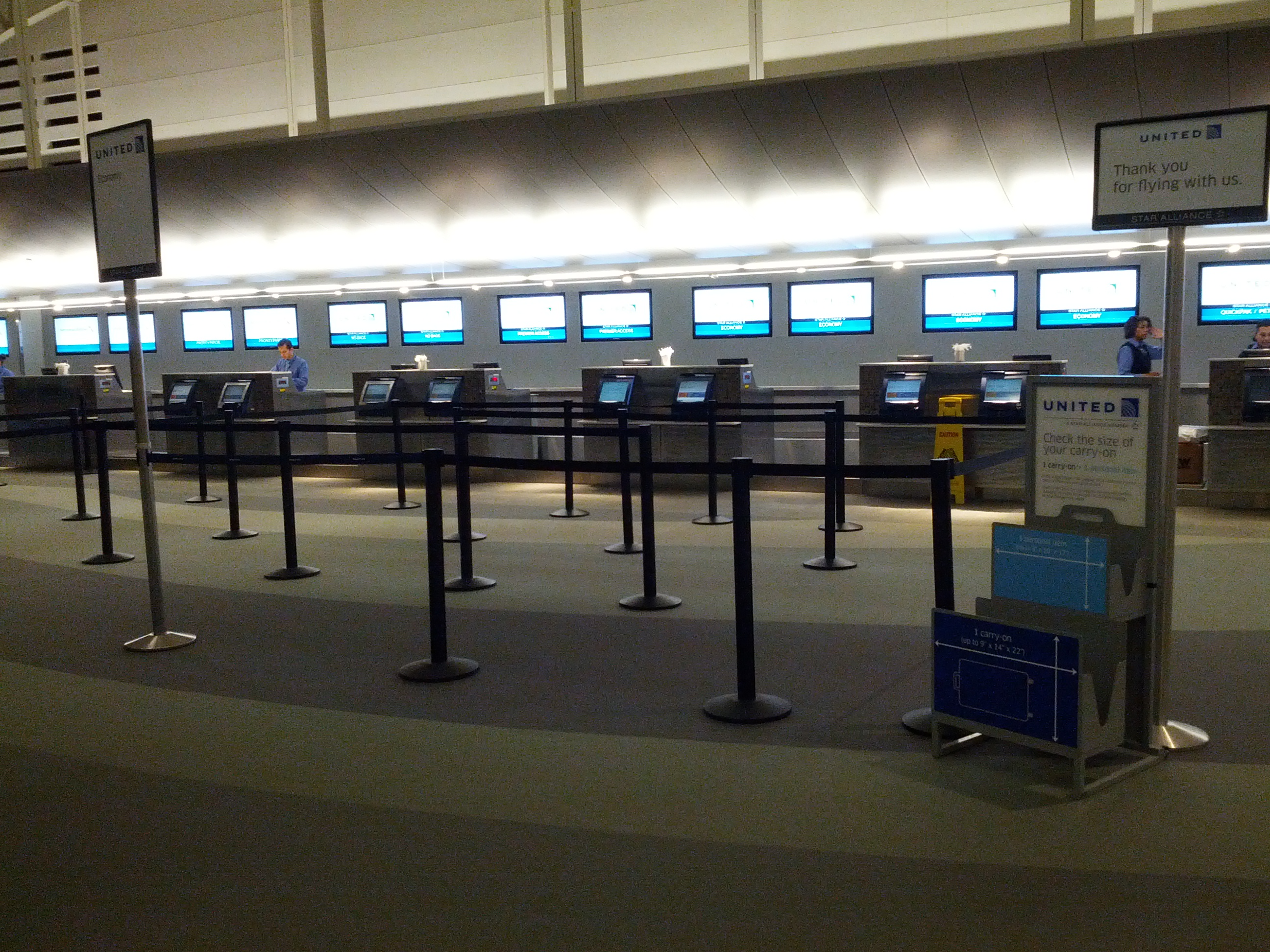
Just to show that this isn’t the norm, here is a view of the lines at the next few airlines… and yes, American is like this too!  Hooray for efficiency!… wait….Â
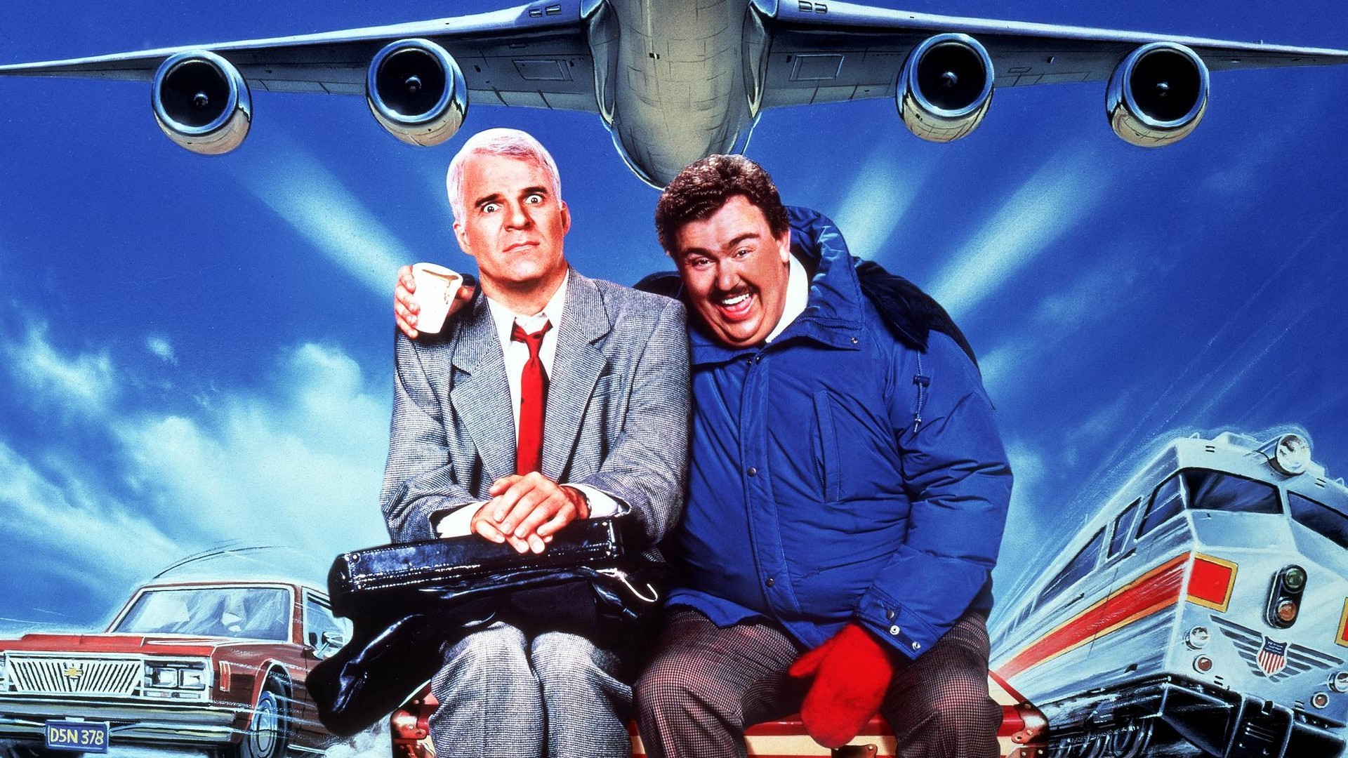
United may break guitars, but they won’t let you miss your flight to check a bag or just print your boarding pass!
Trains 1: Leg 3: DCA to Union Station
I’ve almost become a DC resident, this is my third time to DC this year. Â I am a card-carrying WMATA rider, as my employer makes me do paperwork to rent a vehicle and for anything to DC they’ll probably (rightly) tell me to take the train. Â I’ve grown accustom to it, and WMATA will probably be happy that I’ll be bringing my card up from -$0.45 to something positive.
I’ve done the Yellow/Blue -> Red line drill many times. Â This will be cake. Â Famous Last Words.
Thank God they didn’t penalize me for being -$0.45… yes, that’s a negative sign! Â I immediately put $5 onto the card which took care of me for the rest of the trip.
Trains 2: Union Station to Penn Station
This is interesting to me because I’ve only been on subways in Chicago, Atlanta, and DC. Â The only surface trains I’ve been on were Chicago (the El) and amusement trains (one north of Cincinnati and virtually every amusement park I’ve been to). Â I’ve never been on a train like the MARC train. Â I don’t know what to expect.
You might be a transportation planner if you know which subways you’ve been on and you look forward to a new experience on a commuter train. Â You might also be a transportation planner if you’ve navigated more than one subway system while inebriated.
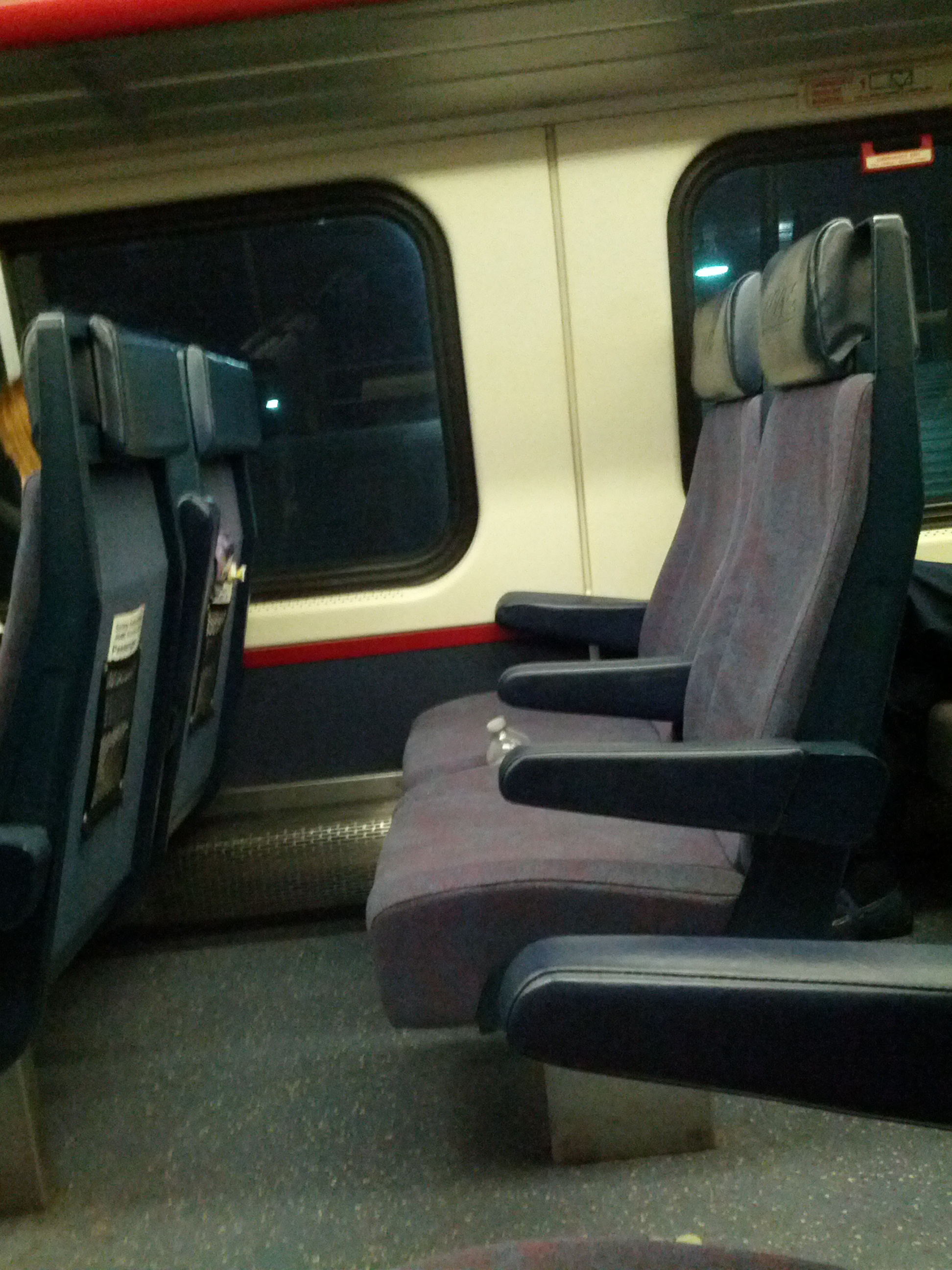
It was interesting to see complaints about these trains on Twitter the day after I returned from ITM. Â There’s legroom and the train was surprisingly smooth and quiet. Â Definitely not what I expected!
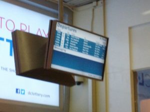
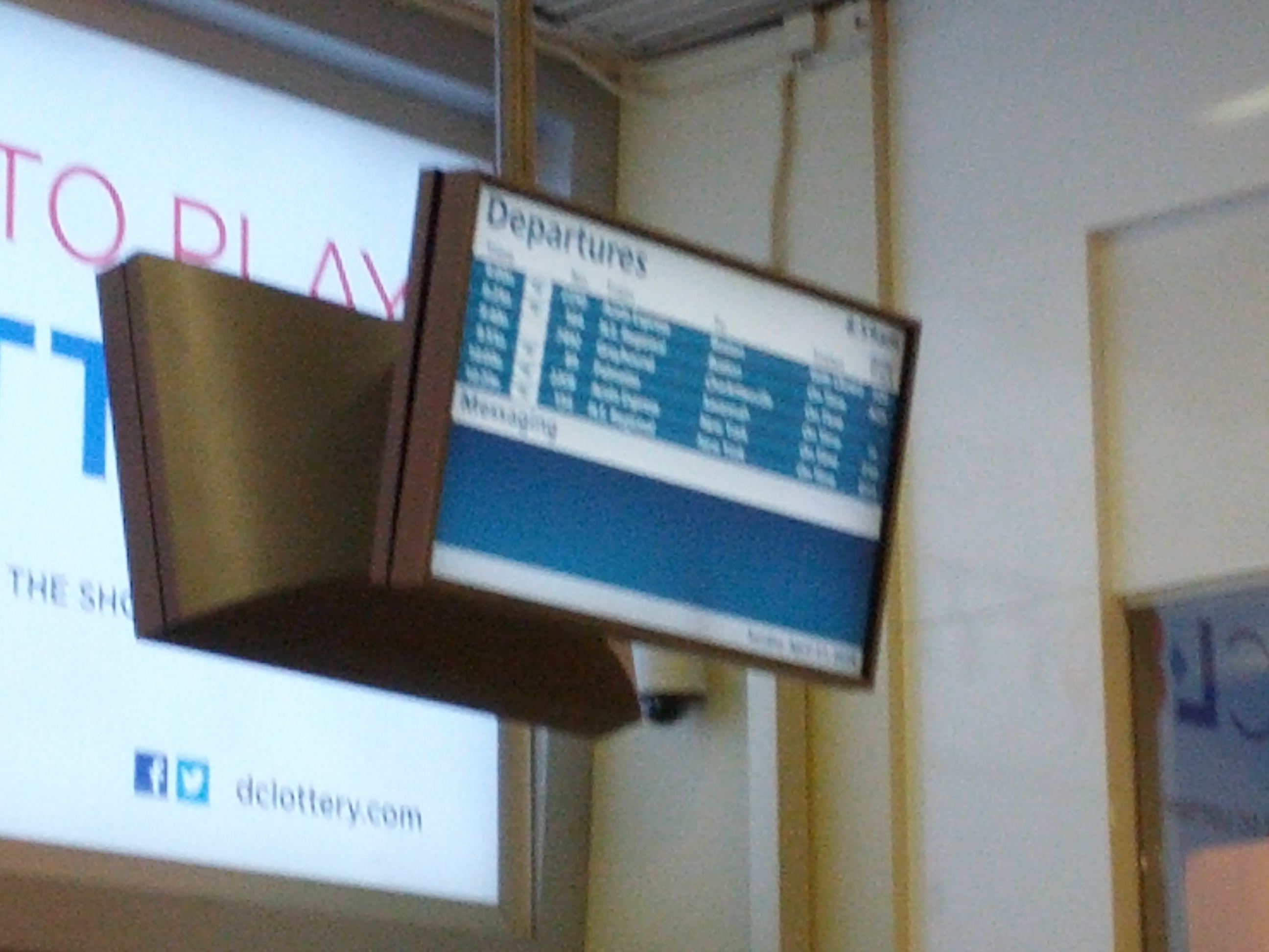
This was interesting to me, as this is my first time in a train station that tells you to use different doors and tracks. I definitely appreciated that they put messages on the bottom of the screen that were basically closed-captions of what was going over the difficult-to-hear loudspeaker!
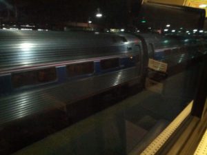
I was on the upper level of a train (cool!) looking down on a smaller train (cool!)

This is as much leg and butt room as first class on an airline. Way more than cattle class!
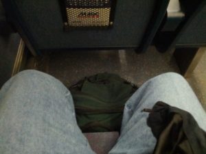
Legroom!!!
Trains 3: Penn Station to Camden Yards
Why stop the streak with a bus now? Â I’m jumping on the light rail. Â Truthfully, there are reasons why. Â I won’t pause riding a bus in Cincinnati to a new area because nothing in Cincinnati is really that new, but not knowing an area, I’d prefer set stops that are announced as opposed to guessing when to pull a stop-request cable to get a bus driver to stop.
I wasn’t even that weirded out by the guy that kept talking to me despite little acknowledgement from me. Â He was a vet and didn’t ask for money, so he wasn’t terrible… but he should probably consider holding off the details of getting busted by the transit police for an outstanding misdemeanor warrant!!!
The Return
Everything you read here went in reverse except the light rail. Â On Tuesday (ITM ended on Wednesday), I got outside to run at about 6:15 AM, and sometime between the end of the run and me coming out of the shower and going downstairs for breakfast it started raining and never did stop. Â So when a gentleman checking out of the hotel next to me asked for a cab to Penn Station, I immediately asked if he wanted to split the fare and he accepted. Â
Pictures
-

-
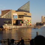
I saw this on my long run on Sunday. I normally won’t stop mid-run to take a picture, but I couldn’t pass this up!
-
-
Submarine. Jimmy Carter served on this vessel.
-
-
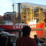
This is a lightship (lighthouse-on-a-ship). While our tour-guide was talking about the lights on top I was noticing the folded-dipole antenna strung between the masts!
-
-
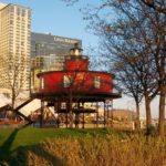
The lighthouse that replaced the lightship in the prior picture.
-
-
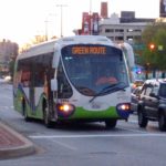
This is the ugly buskling. A colleague actually said he was going to make sure his local transit agency does not order buses this ugly!
-
-
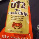
Crab-seasoned potato chips. Not bad if eating a few, but the spice got to me a little and I didn’t finish the bag.
-

-
Two consultants that I originally saw looking very tired. They are laughing at me in this pic because my phone took FOREVER to switch to the camera to take this pic!
-
-
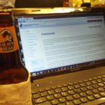
Hacking night. Our hacking is fueled by good beer!
-
-
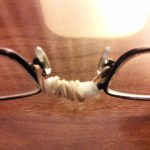
Tuesday night (it was raining). I went to dinner with several others and when wiping the rainwater off my glasses, they snapped. Needless to say, Thursday morning (after the conference) included getting new glasses!
Blog Preview
Coming up on the blog, not sure in what order:
- Race Reports for the Little King’s 1 Mile and the Flying Pig Half Marathon
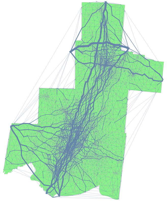
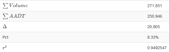
- GPS Survey Processing and Additional Investigations
- Innovations Conference Recap
- ISLR Fridays starting sometime soon


You must be logged in to post a comment.